US8301537B1 - System and method for estimating portfolio risk using an infinitely divisible distribution - Google Patents
System and method for estimating portfolio risk using an infinitely divisible distribution Download PDFInfo
- Publication number
- US8301537B1 US8301537B1 US13/032,600 US201113032600A US8301537B1 US 8301537 B1 US8301537 B1 US 8301537B1 US 201113032600 A US201113032600 A US 201113032600A US 8301537 B1 US8301537 B1 US 8301537B1
- Authority
- US
- United States
- Prior art keywords
- risk
- parameters
- portfolio
- scenarios
- distribution
- Prior art date
- Legal status (The legal status is an assumption and is not a legal conclusion. Google has not performed a legal analysis and makes no representation as to the accuracy of the status listed.)
- Active, expires
Links
Images


Classifications
-
- G—PHYSICS
- G06—COMPUTING; CALCULATING OR COUNTING
- G06Q—INFORMATION AND COMMUNICATION TECHNOLOGY [ICT] SPECIALLY ADAPTED FOR ADMINISTRATIVE, COMMERCIAL, FINANCIAL, MANAGERIAL OR SUPERVISORY PURPOSES; SYSTEMS OR METHODS SPECIALLY ADAPTED FOR ADMINISTRATIVE, COMMERCIAL, FINANCIAL, MANAGERIAL OR SUPERVISORY PURPOSES, NOT OTHERWISE PROVIDED FOR
- G06Q40/00—Finance; Insurance; Tax strategies; Processing of corporate or income taxes
- G06Q40/06—Asset management; Financial planning or analysis
Definitions
- the present invention relates in general to financial portfolio management and, specifically, to a system and method for estimating portfolio risk using an infinitely divisible distribution.
- a probability distribution is considered leptokurtic if the distribution exhibits Kurtosis, where the mass of the distribution is greater in the tails and is less in the center or body, when compared to a Normal distribution.
- a probability distribution can be considered asymmetric if one side of the distribution is not a mirror image of the other side, when the distribution is divided at the maximum value point or the mean.
- volatility clustering that is, calm periods, which are followed by highly volatile periods or vice versa.
- the stable Paretian distribution also has the appealing property that the stable Paretian distributions is the only distribution that arises as a limiting distribution of sums of independently, identically distributed (iid) random variables. This is required when error terms are assumed to be the sum of all external effects that are not captured by the model.
- the drawbacks and limitations of the previous approaches to financial market modeling are overcome by the system and method described herein.
- the system achieves maximum statistical reliability, statistical model accuracy, and predictive power in order to achieve market consistent derivative pricing.
- the system provides the required behavior in two respects. First, scenarios for future market prices and value at risk are accurately predicted. Second, arbitrage-free prices of derivatives are produced, in the risk neutral world.
- the system employs a infinitely divisible distribution which allows the leptokurtic property, asymmetry, and existence of arbitrary moments and the exponential moment for all real line.
- a synthetic Tempered Stable (SynTS) distribution is one example of the infinitely divisible distribution.
- the synthetic Tempered Stable distribution is obtained by taking an ⁇ -stable law and multiplying the Levy measure by the rapidly decreasing functions onto each half of the real axis.
- the rapidly decreasing Tempered Stable (RDTS) distribution, exponentially tilted rapidly decreasing Tempered Stable distribution, and generalized rapidly decreasing Tempered Stable distribution are subclasses of the synthetic Tempered Stable distribution.
- the infinitely divisible distributions can be implemented for univariate or multivariate cases.
- the stochastic process models employed herein are based on three main components: (1) A general multivariate time series process, such as the ARMA-GARCH family; (2) an innovation process where the marginal of the probability distribution follow an infinitely divisible distribution; (3) and a dependence structure model which could be based on two approaches: (3.1) a copula approach to model the dependence structure between the risk factors; (3.2) and a subordinated model representation of the infinitely divisible distribution.
- a multivariate time series model such as the ARMA-GARCH family
- ARMA-GARCH multivariate time series model
- Some subclasses of infinitely divisible distributions e.g. RDTS, or SynTS distribution
- RDTS RDTS
- SynTS SynTS distribution
- the use of either a copula approach or subordinate model representation combine modeling flexibility with computational tractability for complex dependency structures. All together the approach leads to a realistic and reliable model to describe the statistical properties of objects in the financial market, for example the return process of stocks or indexes, the term structure of interest rates, and the defaultable firm values.
- the first step is a multivariate stochastic process describing the joint dynamics of different risk factors including, returns of individual securities, returns of appropriate market indices, various types of yield curves, exchange rates, interest rates, and default probability.
- the model parameters for the system can be calibrated to a set of exogenously provided derivative prices.
- the system calculates risk measures and determines prices of derivatives including options and swaps. Calculated risk measures can then be used for portfolio optimization.
- One embodiment provides a system and method for estimating portfolio risk using an infinitely divisible distribution.
- a time series comprising a plurality of risk factors applicable over at least one time horizon, a portfolio comprising a plurality of financial assets, and one or more risk adjusted return points for the financial assets are stored.
- the financial assets are associated with the risk factors.
- the parameters of one or more risk factors such as financial returns series are estimated based on an infinitely divisible tempered stable distribution model exhibiting leptokurtic behavior. Scenarios are generated for the model. One of Value at Risk, Average Value at Risk, and their derivatives are then determined.
- FIG. 1 is a functional block diagram showing a system for estimating portfolio risk using an infinitely divisible distribution, in accordance with one embodiment.
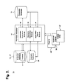
- FIG. 2 is a block diagram showing a portfolio modeler for use in the system of FIG. 1 .
- FIG. 3 is a block diagram showing a parameter estimation module for use in the portfolio modeler of FIG. 2 .
- FIG. 4 is a block diagram showing a scenario generation module for use in the portfolio modeler of FIG. 2 .
- FIG. 5 is a block diagram showing an application object module for use in the portfolio modeler of FIG. 2 .
- FIG. 6 is a flow diagram showing a method for market parameter estimation, in accordance with one embodiment.
- FIG. 7 is a flow diagram showing a method for risk-neutral parameter estimation, in accordance with one embodiment.
- FIG. 8 is a flow diagram showing a method for generating market scenarios, in accordance with one embodiment.
- FIG. 9 is a flow diagram showing a method for generating risk-neutral scenarios, in accordance with one embodiment.
- FIG. 1 is a functional block diagram 9 showing a system 10 for estimating portfolio risk using an infinitely divisible distribution, in accordance with one embodiment.
- a workstation 11 is interoperatively interfaced to a plurality of servers 12 - 14 over a network 18 , which can include an internetwork, such as the Internet, intranetwork, or combination of networking segments.
- the workstation 11 operates as a stand-alone determiner system without interfacing directly to other determiner systems, although data can still be exchanged indirectly through file transfer over removable media.
- Other network domain topologies, organizations and arrangements are possible.
- the workstation 11 includes a portfolio modeler (PM) 19 that generates the vectors and estimates portfolio risk for a portfolio of financial assets 20 , as further described below beginning with reference to FIG. 2 .
- the servers 12 - 14 each maintain a database 15 - 17 containing financial data, such as historical record of securities and risk factors for securities, that can optionally be retrieved by the workstation 11 during parameter estimation, scenario generation, risk calculation, risk budgeting, portfolio optimization, and portfolio reoptimization.
- the portfolio 20 can include one or more financial assets, including securities and other forms of valuated properties, such as described in Fabozzi, F. J., “The Theory & Practice of Investment Management,” Chs. 1-2, pp.
- a portfolio 20 with a flat structure is optimized, where all assets, regardless of type, are in the same portfolio.
- each portfolio 20 can be composed of any number of subportfolios, which can also be composed of subportfolios to any depth of hierarchy.
- a subportfolio can be used, for instance, to contain any set of financial assets 26 convenient to the user or portfolio manager.
- a user or portfolio manager may decide to create subportfolios, which segregate the overall portfolio by asset type or class.
- the optimization can be done within each subportfolio and across the collections of portfolios at any level in the hierarchy.
- the time horizon of the optimization can be different for each level of portfolio and subportfolio.
- the individual determiner systems including the workstation 11 and servers 12 - 14 , are general purpose, programmed digital determining devices consisting of a central processing unit (CPU), random access memory (RAM), non-volatile secondary storage, such as a hard drive or CD ROM drive, network interfaces, and can include peripheral devices, such as user interfacing means, such as a keyboard and display.
- Program code including software programs, and data are loaded into the RAM for execution and processing by the CPU and results are generated for display, output, transmittal, or storage.
- FIG. 2 is a block diagram 30 showing a portfolio modeler 19 for use in the system 10 of FIG. 1 .
- the portfolio modeler 19 estimates financial risk and valuation of derivatives by utilizing a class of infinitely divisible distributions and time series models based on the infinitely divisible distribution and optimizes risk adjusted return for the portfolio 31 of financial assets.
- the portfolio modeler 19 includes components, or modules, for estimating parameters 32 and generating scenarios 33 , and one or more application object modules 34 to calculate portfolio risk, portfolio optimization, and option pricing.
- the portfolio optimizer 19 maintains one or more databases in which historical and generated financial data and variables, such as observation data and associated dates, time windows for selecting financial data sample size is stored. Other stored data is possible, including risk factors, risk free rates, benchmark returns, asset allocation weights, and risk adjusted returns.
- the portfolio modeler 19 can generate output data such as risk factor scenarios, option pricing, and portfolio optimization results, graphical displays 38 , such as an efficient frontier graph, and reports 39 , such as a risk report or tabular report of an optimized portfolio or scenarios. Other forms of output are possible.
- the parameter estimation module 32 reads returns of individual securities, returns of appropriate market indices, various types of yield curves, exchange rates, interest rates, default probability, and derivatives prices including options and futures. The parameter estimation module 32 then estimates market parameters and risk-neutral parameters for infinitely divisible models with time varying volatility, as further described below with reference to FIG. 3 .
- An example of the infinitely divisible model with time varying volatility is the ARMAX-GARCH model with univariate and multivariate infinitely divisible distributed innovations. Estimated parameters are saved in the parameter database 35 , on a regular basis, such as everyday.
- the scenario generation module 33 generates scenarios using the estimated parameters, as further described below with reference to FIG. 4 .
- the scenario generation module 33 forecasts future probability distribution of asset returns based on the infinitely divisible model with time varying volatility using parameters estimated and saved by parameter estimation module 32 .
- the scenario generation module 33 generates simulated future scenario of market volatility process, market return process, risk-neutral volatility process, and risk-neutral return process. Generated processes are saved in a scenario database 36 .
- the application object modules 34 utilize various applications using the estimated parameters and generated scenarios, as further described below with reference to FIG. 5 .
- the major application objects are value at risk (VaR) and average value at risk (AVaR) calculators and European/American type option price calculator. Portfolio optimization can be then be carried out using the VaR and AVaR calculator.
- FIG. 3 is a block diagram 40 showing a parameter estimation module 32 for use in the portfolio modeler 19 of FIG. 2 .
- the parameter estimation module 32 reads returns of individual securities, market indexes (i.e. returns of appropriate market indices, various types of yield curves, exchange rates, interest rates, and default probability), and derivatives prices including options and futures from a financial database 15 - 17 and then estimates ARMAX-GARCH model parameters and infinitely divisible model parameters. Estimated parameters are the stored in the parameter database 35 .
- the market parameter estimation includes a ARMAX-GARCH parameter estimator 41 and a Fat-tail and tail dependency estimator.
- the ARMAX-GARCH parameter estimator 41 estimates ARMAX-GARCH model parameters using returns of individual securities and market indexes, and then generate a residual time-series 43 .
- the Fat-tail and tail dependency estimator 42 estimates parameters of infinitely divisible distributions and dependence structure using the residual 43 and parameters estimated by the ARMAX-GARCH parameter estimator 41 . In one embodiment the ARMAX-GARCH is omitted.
- the ARMAX-GARCH parameter estimator 41 can include only the ARMA or the GARCH component of the ARMAX-GARCH model.
- Parameters of infinitely divisible distributions are modeled by various tempered stable and tempered infinitely divisible distributions, as further described below in the section titled Infinitely Divisible Distribution.
- the dependence structure can be modeled in two ways, by a copula method and or by a sub-Gaussian (GRDTS) model as further described below in the section titled Multi-dimensional Consideration.
- the risk-neutral parameter estimation portion estimates risk-neutral parameters of an infinitely divisible model using derivatives prices and market parameters estimated in the market parameter estimation portion.
- the risk neutral parameters deduce an equivalent martingale measure (EMM), which is a martingale measure equivalent to the market measure generated by the market infinitely divisible parameters.
- EMM equivalent martingale measure
- risk neutral parameters can be estimated using the derivative prices. In one embodiment, first, fix ARMAX-GARCH parameters estimated using market stock prices. In other embodiments the ARMAX-GARCH component is skipped. Next, calibrate risk neutral parameters. In order to estimate risk neutral parameters, two methods can be used.
- the first is using market price of derivatives (for example European options) and the second is using mathematical theory for finding EMM.
- the risk neutral parameters are calibrated by minimizing distance between theoretical derivative prices and market prices. The square root error can be used as the distance.
- the theoretical price can be calculated by the Monte-Carlo simulation method. If there is no data for the derivatives, then the second method is used. Risk neutral parameters satisfying conditions of Theorem 1, Proposition 1, or Corollary 1 to be used, as described further in detail below.
- the method of the market parameter estimation portion and the method of the risk-neutral parameter estimation portion are further described below with reference to FIG. 5 and FIG. 6 , respectively.
- the ARMAX-GARCH model and infinitely divisible models considered in this module are explained in further described below in the section titled ARMAX-GARCH process and the section Infinitely Divisible Distribution, respectively.
- FIG. 4 is a block diagram 50 showing a scenario generation module 33 for use in the portfolio modeler 19 of FIG. 2 .
- the scenario generation module 33 reads ARMAX-GARCH model parameters, infinitely divisible model parameters, and risk-neutral parameters estimated by the parameter estimation module 32 from the parameter database 35 .
- the scenario generation module 33 then forecasts future volatility and simulating future return processes.
- the scenario generation module 33 generates market scenarios and risk-neutral scenarios. Market scenarios are generated by a market return processes generator 51 and risk-neutral scenarios are generated by a risk-neutral return processes generator 52 .
- Infinitely divisible random number can be generated by an inverse transform algorithm or series representation method.
- the inverse transform algorithm uses inverse function of cumulative distribution function to generate the random numbers. Inverse function of the cumulative distribution function for given infinitely divisible distribution is taken. Next, uniformly distributed random numbers are put into the inverse function and then the random number for a given infinitely divisible distribution is obtained.
- the cumulative distribution function for infinitely divisible distribution is described further below in relation to Proposition 2.
- Series representation for the RDTS distribution can be simulated by Theorem 2.
- the method of the market return processes generator 51 and the method of the risk-neutral return processes generator 52 are further described below with reference to FIG. 7 and FIG. 8 , respectively.
- the ARMAX-GARCH model and infinitely divisible models considered in this module are explained in further described below in the section titled ARMAX-GARCH process and the section Infinitely Divisible Distribution, respectively.
- FIG. 5 is a block diagram 60 showing an application object module 34 for use in the portfolio modeler 19 of FIG. 2 .
- VaR and AVaR object 61 is used to calculate VaR and AVaR from the market ARMAX-GARCH parameters and market infinitely divisible parameters in the parameter database 35 . More detail regarding calculating VaR and AVaR with the parametric method is described further below in the section titled Implementation: Calculating VaR and AVaR.
- the simulated scenarios stored in the scenarion database 36 can be used to calculate portfolio VaR and AVaR.
- Portfolio Optimization object 62 is implemented using parameters and scenarios from the parameter database 35 and the scenarion database 36 .
- VaR and AVaR object 61 are partially used to measure portfolio risk and minimize the risk.
- European option and American option 63 object is used to calculate prices of European and American options, respectively.
- the objects use risk neutral parameters from the parameter database 35 and simulated risk-neutral scenario from the scenarion database 36 . More details for option pricing are described further below in the section Implementation: Pricing Derivatives.
- An example of European option pricing under ARMAX-GARCH model with infinitely divisible innovations is provided in the section Example: Pricing call options under the GARCH model with RDTS distributed innovations.
- a derivative also known as a contingent claim, is a financial contract whose values depends on the value of other, more basic underlying variables, called “underlyings”.
- the underlyings can be individual securities, securities indexes or virtually any other variable including interest rates, credit defaults, foreign exchange rates, commodity prices, weather, crop yields, or virtually any other price or a function of these quantities.
- Futures, swaps and options are examples of derivatives.
- a stock option is a derivative whose value is contingent on the (underlying) price of the stock. At the same time, the stock itself can be viewed as a contingent claim on the value of the firm issuing the stock.
- a “call” option gives the holder the right but not the obligation to buy, and a “put” option gives the holder the right but not the obligation to sell.
- the date in the contract is the “expiration date” or “maturity”. If the option allows exercise before the maturity date, then it is “American” style option, but if the option allows exercise only at the maturity, then it is “European” style option.
- the rising cash flow, when the option holders exercise their right is the “payoff”. For example, when a payoff is given by the difference between the current stock price and some fixed price, the fixed price in the contract is the “exercise” or “strike” price.
- a “real option” is a derivative whose “underlyings” are real world asset as opposed to financial assets. Real assets include land, plant, machinery, and so forth. Options can be embedded in investment projects; some examples are an abandonment option, an expansion option, a contraction option, an option to defer, and an option to extend. Other options are also possible.
- the system uses time series processes with Infinitely Divisible innovations for the calculation of probability distributions of financial returns of risk factors.
- the risk factors can be the market price returns of individual financial assets or securities themselves or of a portfolio of financial assets.
- risk factors can be derived as computed values, perhaps from fundamental securities information, or they can be an exogenous factor, such as interest rates or macroeconomic factors, which may affect the price of a security.
- the term return can refer to the relative change in any risk factor over some time horizon or time period.
- a random variable Y is called infinitely divisible if, for each n ⁇ N , there are iid random variables
- )v(dx) ⁇ . If Y is infinitely divisible, then the characteristic function ⁇ Y (u) E[e in Y ] is given by the -Khintchine formula:
- ⁇ is such that ⁇ tilde over ( ⁇ ) ⁇
- An embodiment will use one of the following distribution for modeling the financial market.
- SynTS synthetic tempered stable
- This embodiment would use the ARMAX-GARCH process described below in section ARMAX-GARCH processes and then the residuals will be modeled with Classical Tempred Stable.
- the GRDTS subordinator with parameter ( ⁇ ,C, ⁇ ,p) is a purely non-Gaussian infinitely divisible random variable T whose characteristic function is given by
- v ⁇ ( dx ) ( C + ⁇ e - ⁇ + 2 ⁇ x 2 / 2 ⁇ 1 x > 0 + C - ⁇ e - ⁇ - 2 ⁇ ⁇ x ⁇ 2 / 2 ⁇ 1 x ⁇ 0 ) ⁇ dx ⁇ x ⁇ ⁇ + 1 , and
- G ⁇ ( x ; ⁇ , ⁇ ) 2 - ⁇ 2 - 1 ⁇ ⁇ ⁇ ⁇ ⁇ ( - ⁇ 2 ) ⁇ ( M ⁇ ( - ⁇ 2 , 1 2 ; x 2 2 ⁇ ⁇ 2 ) - 1 ) + 2 - ⁇ 2 - 1 2 ⁇ ⁇ ⁇ - 1 ⁇ x ⁇ ⁇ ⁇ ⁇ ( 1 - ⁇ 2 ) ⁇ M ⁇ ( 1 - ⁇ 2 , 3 2 ; x 2 2 ⁇ ⁇ 2 ) , and M is the Kummer's function or the confluent hypergeometric function as described in Andrews, L.
- L RDTS log-Laplace transform
- the parameter ⁇ determines the path behavior; that is, the RDTS process has finite variation if ⁇ 1 and infinite variation if ⁇ >1.
- ⁇ ⁇ ( x ) 1 2 ⁇ ( ⁇ + 2 - ⁇ ⁇ + 2 ) ⁇ x 2 ⁇ 1 x > 0 + 1 2 ⁇ ( ⁇ - 2 - ⁇ ⁇ - 2 ) ⁇ ( - x ) 2 ⁇ 1 x ⁇ 0 .
- Y t denotes the dependent variable
- X t (X t (1) , X t (2) , . . . , X t (d) ) a vector of exogenous variables.
- the process includes an autoregressive term of length n, a moving average term of length m.
- the measurable function f embodies a generalized ARCH-in mean term, which allows for a non-linear influence of the volatility/variance in the conditional mean equation.
- the innovation process ( ⁇ I ) I ⁇ is assumed to independent and identically distributed (iid) with zero mean and unit variance.
- the time dependent volatility is modeled with the help of a GARCH(p,q) process:
- the multivariate dependency can be constructed by a copula function.
- the marginal evolution of every risk factor is modeled according to equation (32) and (33), and the dependence structure is introduced by a copula function C which describes the joint distribution of the N-dimensional innovation vector ⁇ l as equation (11).
- the multivariate dependency will be generated by using a vector ARMAX-GARCH process of the following form (for simplicity only the the ARCH(1)-process in the bivariate case is shown, but those skilled in the art will understand the simple extension of this formulation to higher dimensional cases):
- [ ⁇ 11 , t ⁇ 21 , t ⁇ 22 , t ] [ ⁇ 11 , t ⁇ 21 , t ⁇ 22 , t ] + [ ⁇ 11 ⁇ 12 ⁇ 13 ⁇ 21 ⁇ 22 ⁇ 23 ⁇ 31 ⁇ 32 ⁇ 33 ] ⁇ [ ⁇ 1 , t - 1 2 ⁇ 1 , t - 1 ⁇ ⁇ 2 , t - 1 ⁇ 2 , t - 1 2 ] ( 34 )
- Some embodiments allow the choice of one or more multivariate dependency structures.
- Other embodiments include facilities to test various possible dependency structures on historical data to determine the structure best suited for the data set. These test facilities may be fully automatic, or fully or partly under the control of a user or operator.
- the marginal distribution of the innovation process is described by infinitely divisible distributions with zero mean and unit variance. Some embodiments will have the standard RDTS distributed innovation, and some other embodiments will have another subclass of the SynTS distributed innovation. Additionally, the foregoing discussion applies equally to other time series processes, such as the ARMA-GARCH and ARIMA-IGARCH families.
- the set of distribution parameters depends on the chosen distribution. For example, within embodiments using standard RDTS or standard ERDTS distributed innovations, there are three distribution parameters per model dimension, and embodiments using standard GRDTS distributed innovations, there are four distribution parameters per model dimension.
- these parameters are simultaneously estimated by means of a numerical conditional maximum likelihood procedure (MLE).
- MLE numerical conditional maximum likelihood procedure
- these parameters are estimated stepwise by a Gaussian conditional maximum-likelihood procedure for the model parameters and, in a second step, the distribution parameters are determined from the empirical residuals.
- Some other embodiments make use of an iterative estimation procedure, where the model and distribution parameter estimation is iterated until some exit criterion is reached.
- the d-exogenous risk factors and their factor loadings in (32) can be determined (estimated) using factor analysis (time-series factor analysis, cross-sectional factor analysis, or statistical factor analysis) that the use of such factor models can lead to significant reduction of the number d of risk factors involved in the estimation of the model parameters.
- factor analysis time-series factor analysis, cross-sectional factor analysis, or statistical factor analysis
- the ARMAX-GARCH processes can be used as models in factor analysis, where the d-exogenous variables explain the systematic risk component while the autoregressive part in (32) together with ( 33 ) describes the idiosyncratic (non-systematic) risk.
- Such an approach is an extension of a time series factor analysis framework.
- f x , ⁇ x , and F x be the density function, the characteristic function, and the cumulative distribution function of a tempered stable random variable X, respectively.
- the characteristic function of a given random variable X is defined by the Fourier transform of the probability density function; that is,
- f X ⁇ ( x ) 1 2 ⁇ ⁇ ⁇ ⁇ ⁇ - ⁇ ⁇ ⁇ e - ⁇ u ⁇ ⁇ i ⁇ ⁇ x ⁇ ⁇ x ⁇ ( u ) ⁇ ⁇ d u .
- Proposition 2 can be applied to the tempered stable distribution as follows:
- AVaR with the significance level ⁇ is
- AVaR ⁇ ⁇ ( X ) 1 ⁇ ⁇ ⁇ 0 ⁇ ⁇ VaR ⁇ ⁇ ( X ) ⁇ d ⁇ ⁇ . . AVaR of the temperes stable distributions can be obtained by the following proposition.
- Proposition 3 Let Y be a random variable for the return of an asset or portfolio. Suppose Y is infinitely divisible and the distribution function of Y is continuous. If there is ⁇ >0 such that
- AVaR ⁇ ⁇ ( Y ) VaR ⁇ ⁇ ( Y ) - e - VaR ⁇ ⁇ ( Y ) ⁇ ⁇ ⁇ ⁇ ⁇ ( ⁇ 0 ⁇ ⁇ e - i ⁇ ⁇ uVaR ⁇ ⁇ ( Y ) ⁇ ⁇ Y ⁇ ( - u + i ⁇ ⁇ ⁇ ) ( - u + i ⁇ ⁇ ⁇ ) 2 ⁇ d u ) . ( 1 )
- Model prices for the financial derivatives are evaluated by the Monte Carlo simulation.
- (S t ) t ⁇ [0,T] be the risk-neutral process for price vector of underlyings related to the given derivative.
- the parameters for generating the sample path of (S t ) t ⁇ [0,T] are estimated by the methods in Section Infinitely divisible distribution.
- _Some embodiments generate the risk-neutral price process of (S t ) t ⁇ [0,T] by applying Theorem 1, while other embodiments generate the risk-neutral price process by applying Proposition 1, or corollary 1.
- random number generating methods and variance reduction techniques can be founded in the extensive literature that addresses Monte-Carlo simulation.
- standard references can include Glasserman, P. (2003), Monte Carlo Method In Financial Engineering, Springer.
- LSMv Least Square Regression method with volatility parameter
- LSM Least Square Regression Method
- the Least Square Regression Method (LSM) was introduced by Longstaff, F. A., and Schwartz, E. S., “Valuing American options by simulation: a simple least-squares approach,” Review of Financial Studies, 14: 113-147 (2001), the disclosure of which is incorporated by reference.
- Longstaff and Schwartz's LSM is constructed under the markov process, and it does not consider the volatility parameter.
- the LSMv considers stock price process and volatility process together in the regression.
- the method used standard RDTS as the distribution of the innovation ⁇ t .
- some embodiments will apply other subclasses of infinitely divisible distributions to the innovation distribution, and the extensions to these cases should be clearly understood by those skilled in the art.
- Some embodiments will have the capabilities to price derivative products with other types of underlying or using the multivariate dependency methodologies discussed previously; the extensions to these cases should again also be clearly understood by those skilled in the art.
- ⁇ t t ⁇ is predictable.
- Proposition 4 there is a measure Q t equivalent to P t such that ⁇ t +k t :stdRDIS( ⁇ , ⁇ tilde over ( ⁇ ) ⁇ + (t), ⁇ tilde over ( ⁇ ) ⁇ ⁇ (t)) on the measure Q t , and hence
- the risk-neutral stock price dynamic is called the the RDTS-GARCH option pricing model.
- the stock price S t at time t>0 is given by
- the call option prices are determined by the Monte Carlo method.
- FIG. 6 is a flow diagram 70 showing a method for market parameter estimation, in accordance with one embodiment.
- Financial data such as returns of individual securities, market indexes (i.e. returns of appropriate market indices, various types of yield curves, exchange rates, interest rates, and default probability), and derivatives prices including options and futures are retrieved from a financial database 15 - 17 (block 71 ).
- ARMAX-GARCH model parameters are then estimated using the maximum likelihood estimation under the assumption of normally distributed residual or Student-t distributed residual (block 72 ).
- the ARMAX-GARCH parameter estimator 41 estimates ARMAX-GARCH model parameters using returns of individual securities and market indexes, and then generate a residual time-series 43 .
- the ARMAX-GARCH model is described above in the section titled ARMAX-GARCH process.
- the historical time-series of the residual is extracted using the financial data and estimated parameters (block 73 ).
- the maximum likelihood estimation is applied again to estimate parameters of infinitely divisible distributions using the extracted historical time-series residual (block 74 ).
- Parameters of infinitely divisible distributions are modeled by various tempered stable and tempered infinitely divisible distributions, as described above in the section titled Infinitely Divisible Distribution.
- the dependence structure is estimated using the extracted residuals or read financial data (block 75 ).
- the dependence structure can be modeled in two ways, by a copula method, such as a skewed t-copula, or by a sub-Gaussian model as described above in the section titled Multi-dimensional Consideration.
- Estimated parameters are the stored in the parameter database 35 (block 76 ).
- FIG. 7 is a flow diagram 80 showing a method for risk-neutral parameter estimation, in accordance with one embodiment. Derivatives prices and market parameters estimated in the market parameter estimation portion, as described above with reference to FIG. 6 , are retrieved. Next, the determination is made whether information of options underlying with the considered financial data, such as stock or index, is available (block 82 ).
- Risk-neutral parameters of an infinitely divisible model are estimated from the retrieved derivatives prices and estimated.
- the risk neutral parameters deduce an equivalent martingale measure (EMM), which is a martingale measure equivalent to the market measure generated by the market infinitely divisible parameters.
- EMM equivalent martingale measure
- risk neutral parameters can be estimated using the derivative prices (block 84 ).
- calibrate risk neutral parameters which minimize the distance between theoretical derivative prices and market prices. For example, the square root error can be used as the distance.
- the theoretical price can be calculated by the Monte-Carlo simulation method.
- the find risk neutral parameter is used such that the measure generated by the risk-neutral measure becomes an EMM, satisfying conditions of Theorem 1, Proposition 1, or Corollary 1, as described above (block 85 ). In either case, the estimated risk-neutral parameters are then stored (block 86 ).
- FIG. 8 is a flow diagram 90 showing a method for generating market scenarios, in accordance with one embodiment.
- ARMA-GARCH model parameters and infinitely divisible model parameters are retrieved from the parameter database 35 (block 91 ).
- scenario, j is set to 1 (block 92 ) and time, t, is set to the current time and T is a parameter of the algorithm which is set equal to the maturity date (block 93 ).
- Future volatility is forecast using the GARCH model (block 94 ).
- An infinitely divisible random number is generated using the infinitely divisible parameter retrieved (block 95 ).
- the infinitely divisible models are described above in the section titled Infinitely Divisible Distribution.
- the infinitely divisible random number can be generated by an inverse transform algorithm or series representation method.
- the inverse transform algorithm uses inverse function of cumulative distribution function to generate the random numbers. Inverse function of the cumulative distribution function for given infinitely divisible distribution is taken. Next, uniformly distributed random numbers are put into the inverse function and then the random number for a given infinitely divisible distribution is obtained.
- the cumulative distribution function for infinitely divisible distribution is described further below in relation to Proposition 2.
- Series representation for the RDTS distribution can be simulated by Theorem 2.
- the future returns are calculated using the ARMAX model with the generated random numbers (block 96 ).
- the future return is put into the j-th scenario at time t.
- the ARMAX-GARCH model is described above in the section titled ARMAX-GARCH process.
- the determination is then made whether t ⁇ T (block 97 ). If so, then T is set to (t+1) day (block 98 ) and the method returns to the forecasting future volatility step (block 94 ). If t is not less than T, then the determination is made whether scenario j is less than the maximum number of scenarios, for example, 110,000 scenarios (block 99 ). If j is less than the maximum number of scenario, then j is set to j+1 (block 100 ) and the method returns to block 93 . If j is not less than the maximum number of scenario, then the market scenarion generated is stored (block 101 ).
- FIG. 9 is a flow diagram 110 showing a method for generating risk-neutral scenarios, in accordance with one embodiment.
- ARMA-GARCH model parameters are retrieved from the parameter database 35 (block 111 ).
- scenario, j is set to 1 (block 112 ) and time, t, is set to the current time and T is a parameter of the algorithm which is set equal to the maturity date (block 113 ).
- Future volatility is forecast using the GARCH model (block 114 ).
- Risk-neutral infinitely divisible parameters which generate equivalent martingale measures are found.
- the find risk-neutral parameter are found such that the measures generated by the risk-neutral measure are equivalent martingale measures, and satisfy conditions of Theorem 1, Proposition 1, or Corollary 1, as described above (block 115 ).
- An infinitely divisible random number is generated using the risk-neutral infinitely divisible parameter found (block 116 ).
- the infinitely divisible models are described above in the section titled Infinitely Divisible Distribution B.
- the infinitely divisible random number can be generated by an inverse transform algorithm or series representation method.
- the inverse transform algorithm uses inverse function of cumulative distribution function to generate the random numbers. Inverse function of the cumulative distribution function for given infinitely divisible distribution is taken. Next, uniformly distributed random numbers are put into the inverse function and then the random number for a given infinitely divisible distribution is obtained.
- the cumulative distribution function for infinitely divisible distribution is described further below in relation to Proposition 2.
- Series representation for the RDTS distribution can be simulated by Theorem 2.
- the future returns are calculated using the ARMAX model with the generated random numbers (block 117 ).
- the future return is put into the j-th scenario at time t.
- the ARMAX-GARCH model is described above in the section titled ARMAX-GARCH process.
- the determination is then made whether t ⁇ T (block 118 ). If so, then T is set to (t+1) day (block 119 ) and the method returns to the forecasting future volatility step (block 114 ). If t is not less than T, then the determination is made whether scenario j is less than the maximum number of scenarios, for example, 110,000 scenarios (block 120 ).
- j is set to j+1 (block 121 ) and the method returns to block 113 . If j is not less than the maximum number of scenario, then the market scenarion generated is stored (block 122 ).
Abstract
Description
where
where A≧0, γ∈ and v is a measure. This triplet (A2,v,γ) is unique and called a Levy triplet of Y. Conversely, for any choice (A2,v,γ) satisfying the conditions above, there exists an infinitely divisible random variable Y whose characteristic function is given as φY.
-
- 1. X0=0 a.s.
- 2. X has independent increments: given 0<t1<t2< . . . <tn, the random variables Xt
1 , Xt2 −Xt1 , . . . , Xtn −Xtn−1 are independent. - 3. X has stationary increment: for t≧0, the distribution of of X1+s−Xs does not depend on s≧0.
- 4. X is stochastically continuous: ∀t≧0 and α>0,
-
- 5. X is right continuous and has left limits.
A2=Ã2, (2)
with the function
and if A2=0 then
When P and Q are equivalent, the Radon-Nikodym derivative is
where (Ut,) is a process in which triplet (AU 2,vU,γU) of (Ut)t∈[0,T] is given by
Here η is such that
{tilde over (γ)}−γ−∫|x|≦1 x({tilde over (v)}−v)(dx)=A 2η
if A>0 and zero if A=0.
v 0(dx)=M 0(dr,du)=r −α−1 dr ζ(du), (7)
where α ∈(0,2), ζ a finite measure on the unit sphere Sd−1, and r>0, u ∈ Sd−1.
v(dx)=M(dr,du)=r −α−1 q(r,u)dr ζ(du), (8)
where q(r,u) is a positive function on (0,∞)×Sd−1 such that limr→0+q(r,u)>0 and limr→∞q(r,u)=0.
-
- 1. If consider
q(r,1)=e −λ+ 2 r2 /2 , q(r,−1)=e −λ− 2 r2 /2, - and
ζ(1)=C +, ζ(−1)=C −
- 1. If consider
-
- 2. If consider
q(r,1)=e βr−λ2 r2 /2 , q(r,−1)=e −βr−λ2 r2 /2, - and
ζ(1)=ζ(−1)=C
- 2. If consider
-
- 3. If consider
q(r,1)=exp(βr−(λ+ r)p), q(r,−1)=exp(−βr−(λ− r)p), and
ζ(1)=C +, ζ(−1)=C −
- 3. If consider
-
- 4. If consider
-
- and
ζ(1)=C +, ζ(−1)=C −
- and
-
- 5. If consider, for λ+, λ−, C+, C−>0
q(r,u)=e −λ+ r1u=1 +e −λ− r1u=−1 and ζ({1})=C +, ζ({−1})=C − - on R, then we obtain the KoBoL or the classical tempered stable (CTS) distribution. If λ+=λ− then we obtain the flight and if C+=C− then we obtain the CGMY distribution. Moreover, if the CTS distribution has zero mean and unit variance, the distribution is called standard CTS distribution. (See Boyarchenko, S. I. and Levendorskii, S. Z., “Option pricing for truncated Levy processes”, International Journal of Theoretical and Applied Finance, 3, (2000); Carr, P., Geman, H., Madan, D., Yor, M., “The fine structure of asset returns: an empirical investigation”, Journal of
Business 75, 305-332, (2002); and Koponen, I, “Analytic approach to the problem of convergence of truncated Levy flights towards the Gaussian stochastic process”, Physical Review E, 52. (1995)) the disclosures of which are incorporated by reference.
- 5. If consider, for λ+, λ−, C+, C−>0
P(X t (1) ≦x 1 , X t (2) ≦x 2 , . . . , X t (N) ≦x N)=C(F 1(x 1), F 2(x 2), . . . , F N(x N)) (11)
where C denotes the copula function and Fi, i=1,2, . . . , N denotes the distribution function of the i-th component of the N-dimensional process.
The N-dimensional Sub-Gaussian GRDTS Model (Type 1):
X=(X 1 , X 2 , . . . , X N)=μ+γ(T−1)+√{square root over (T)}Z,
-
- where
- μ=(μ1, μ2, . . . , μN)∈ RN, γ=(γ1, γ2, . . . , γN)∈ RN,
- Z=(Z1, Z2, . . . , ZN)˜N(0,Σ), Σ=[σk,l]k,l∈{1,2, . . . ,N}
- T:1-dim GRDTS subordinator with parameter (α,C,θ,p)
The N-dimensional Sub-Gaussian GRDTS Model (Type 2):
X=(X 1 , X 2 , . . . , X N)=μ+γ·(T−1)+√{square root over (T)}·Z, - where
- 1=(1,1, . . . 1) ∈ RN,
- μ=(μ1, μ2, . . . , μN) ∈ RN,
- γ=(γ1, γ2, . . . , γN) ∈ RN,
- Z=(Z1, Z2, . . . , ZN)˜N(0,Σ), Σ=[σk,l]k,l∈{1,2, . . . ,N}
- T=(T1, T2, . . . , TN),
- Tk:TID subordinator with parameter (αk, Ck, θk, pk), k ∈{1,2, . . . , N}
- Tk and Tl are independent for all k,l ∈{1,2, . . . , N}.
The N-dimensional Sub-Gaussian GRDTS Model (Type 3): - where
X=(X 1 , X 2 , . . . , X N)=μ+γ·(T*−1)+√{square root over (T)}·Z, - 1=(1,1, . . . 1) ∈ RN,
- μ=(μ1, μ2, . . . , μN) ∈ RN,
- γ=(γ1, γ2, . . . , γN) ∈ RN,
- Z=(Z1, Z2, . . . , ZN)˜N(0,Σ), Σ=[σk,l]k,l∈{1,2, . . . ,N}
- T*=(T*1, T*N, . . . , T*N),
- T=(T1, T2, . . . , TN),
- T*k:GRDTS subordinator with parameter (α*k, C*k, θ*k, p*k), k ∈{1,2, . . . , N}
- Tk:GRDTS subordinator with parameter (αk, Ck, θk, pk), k ∈{1,2, . . . , N}
A=0,
and
φ(u)=exp(ium+C + G(iu;α,λ +)+C − G(−iu;α,λ −)) (12)
where
and M is the Kummer's function or the confluent hypergeometric function as described in Andrews, L. D., “Special Functions Of Mathematics For Engineers”, Oxford University Press, 2nd edition (1998), the disclosure of which is incorporated by reference. The Laplace transform is defined for all real numbers (i.e. E[eθX]<∞ for all θ∈R) and have the explicit formula as
E[e θX]=exp(θm+C + G(θ;α,λ+)+C − G(−θ;α,λ−)). (13)
of X are given by
then X˜RDTS(α,C,C,λ+,λ−,m0) has zero mean and unit variance, and X will be called the standard RDTS distribution and denoted by X˜stdRDTS(α, λ+, λ−). Moreover, the log-Laplace transform of X will be denoted by LRDTS(x; α, λ+, λ−). By equation (13), the function LRDTS(x; α, λ+, λ−) is finite for all x ∈ R, and then
L RDTS(x;α,λ +,λ−)=m 0 x+C(G(x;α,λ +)+G(−x;α,λ −)). (15)
converges a.s.. Furthermore, that X˜RDTS(α,C,C,λ+,λ−,0).
where (Ut,P) is a process with triplet (AU 2, VU, γU) given by
where
where Yt denotes the dependent variable, Xt=(Xt (1), Xt (2), . . . , Xt (d)) a vector of exogenous variables. The process includes an autoregressive term of length n, a moving average term of length m. The measurable function f embodies a generalized ARCH-in mean term, which allows for a non-linear influence of the volatility/variance in the conditional mean equation. In the present embodiment, the innovation process (εI)I∈ is assumed to independent and identically distributed (iid) with zero mean and unit variance. The time dependent volatility is modeled with the help of a GARCH(p,q) process:
-
- d+1 parameters for the constant term and the exogenous variables;
- n autoregressive terms;
- m moving average terms, and;
- p+q+1 GARCH parameters.
where
VaRε(X)=−inf{y ∈ R:P(X≦y)≦ε}
If Fx(x) is continuous, then we have VaRε(X)=−Fx −1(ε). The definition of AVaR with the significance level η is
AVaR of the temperes stable distributions can be obtained by the following proposition.
AVaRt,η(y i+1)=−(c+ay t +bσ tεt)+σt+1
and
Vart,η(y t+1)=−(c+ay t +bσ tεt)+σt+1
for Monte-Carlo simulation.
where St is the stock price at time t, rt and dt denote the risk-free and dividend rate for the period [t−1,t], respectively, and λt is defined at the time t−1 and can be interpreted as the market price of risk. S0 is the present observed price. The function L(x) is the log-Laplace-transform of εt, i.e, L(x)=log(E[exε
σt 2=(α0+α1σt−1 2εt−1 2+β1σt−1 2), t ∈ N, ε 0=0, (38)
where α0, α1 and β1 are non-negative, α1+β1<1, and α0>0. Clearly the process (σt)t∈ is predictable.
where kt is equal to equation (40). By Proposition 4, there is a measure Qt equivalent to Pt such that εt+kt:stdRDIS(α,{tilde over (λ)}+(t),{tilde over (λ)}−(t)) on the measure Qt, and hence
where ξt:stdRDTS(α,{tilde over (λ)}+(t),{tilde over (λ)}−(t)). Since λtσt disappears in the dynamic on Qt, the variable λt can be interpreted as the market price of risk. Consequently, deduce a risk-neutral stock price dynamic from Proposition 4 as follows:
having the following variance process
σt 2=(α0+α1σt−1 2(ξt−1 −k t−1)2+β1σt−1 2). (42)
be equal to equation (41).
Claims (20)
v(dx)=M(dr,du)=r −α−1 q(r,u)dr ζ(du),
v(dx)=M(dr,du)=r −α−1 q(r,u)dr ζ(du),
X=(X 1 , X 2 , . . . , X N)=μ+γ(T−1)+√{square root over (T)}Z,
X=(X 1 , X 2 , . . . , X N)=μ+γ(T−1)+√{square root over (T)}Z,
Priority Applications (1)
| Application Number | Priority Date | Filing Date | Title |
|---|---|---|---|
| US13/032,600 US8301537B1 (en) | 2010-02-22 | 2011-02-22 | System and method for estimating portfolio risk using an infinitely divisible distribution |
Applications Claiming Priority (2)
| Application Number | Priority Date | Filing Date | Title |
|---|---|---|---|
| US30655710P | 2010-02-22 | 2010-02-22 | |
| US13/032,600 US8301537B1 (en) | 2010-02-22 | 2011-02-22 | System and method for estimating portfolio risk using an infinitely divisible distribution |
Publications (1)
| Publication Number | Publication Date |
|---|---|
| US8301537B1 true US8301537B1 (en) | 2012-10-30 |
Family
ID=47045853
Family Applications (1)
| Application Number | Title | Priority Date | Filing Date |
|---|---|---|---|
| US13/032,600 Active 2031-04-23 US8301537B1 (en) | 2010-02-22 | 2011-02-22 | System and method for estimating portfolio risk using an infinitely divisible distribution |
Country Status (1)
| Country | Link |
|---|---|
| US (1) | US8301537B1 (en) |
Cited By (14)
| Publication number | Priority date | Publication date | Assignee | Title |
|---|---|---|---|---|
| US20110167020A1 (en) * | 2010-01-06 | 2011-07-07 | Zhiping Yang | Hybrid Simulation Methodologies To Simulate Risk Factors |
| US20140214722A1 (en) * | 2013-01-25 | 2014-07-31 | The Research Foundation Of The State University Of New York | Real time evaluation of financial returns based on nearly elliptical models |
| US20140282034A1 (en) * | 2013-03-15 | 2014-09-18 | Hewlett-Packard Development Company, L.P. | Data analysis in a network |
| US20150046313A1 (en) * | 2013-08-01 | 2015-02-12 | Thomas LeRoy Pantelis | Distributed software system and communications terminal to increase situational awareness in derivatives trading |
| US20150379643A1 (en) * | 2014-06-27 | 2015-12-31 | Chicago Mercantile Exchange Inc. | Interest Rate Swap Compression |
| US20160019478A1 (en) * | 2014-07-18 | 2016-01-21 | Caterpillar Inc. | Option-based disruption mitigation system in a logistics network |
| US10319032B2 (en) | 2014-05-09 | 2019-06-11 | Chicago Mercantile Exchange Inc. | Coupon blending of a swap portfolio |
| US10475123B2 (en) | 2014-03-17 | 2019-11-12 | Chicago Mercantile Exchange Inc. | Coupon blending of swap portfolio |
| US20190370705A1 (en) * | 2018-06-04 | 2019-12-05 | Jerome lawrence Kreuser | Methods and tools to mitigate financial crashes and advantage financial rallies |
| US10609172B1 (en) | 2017-04-27 | 2020-03-31 | Chicago Mercantile Exchange Inc. | Adaptive compression of stored data |
| US10789588B2 (en) | 2014-10-31 | 2020-09-29 | Chicago Mercantile Exchange Inc. | Generating a blended FX portfolio |
| US11195232B2 (en) | 2016-05-09 | 2021-12-07 | Axioma, Inc. | Methods and apparatus employing hierarchical conditional value at risk to minimize downside risk of a multi-asset class portfolio and improved graphical user interface |
| US11410042B2 (en) | 2018-10-31 | 2022-08-09 | International Business Machines Corporation | Dynamic Boltzmann machine for estimating time-varying second moment |
| US11907207B1 (en) | 2021-10-12 | 2024-02-20 | Chicago Mercantile Exchange Inc. | Compression of fluctuating data |
Citations (6)
| Publication number | Priority date | Publication date | Assignee | Title |
|---|---|---|---|---|
| US6125355A (en) * | 1997-12-02 | 2000-09-26 | Financial Engines, Inc. | Pricing module for financial advisory system |
| US6643631B1 (en) * | 1999-12-17 | 2003-11-04 | The Trustees Of Columbia University In The City Of New York | Method and system for modeling financial markets and assets using fractal activity time |
| US20040172355A1 (en) * | 2003-02-06 | 2004-09-02 | Pandher Gurupdesh S. | Option valuation method and apparatus |
| US7236953B1 (en) * | 2000-08-18 | 2007-06-26 | Athena Capital Advisors, Inc. | Deriving a probability distribution of a value of an asset at a future time |
| US7349878B1 (en) * | 1996-08-16 | 2008-03-25 | Options Technology Company, Inc. | Simulation method and system for the valuation of derivative financial instruments |
| US7599870B2 (en) * | 2002-04-12 | 2009-10-06 | Glo Software Llc | System, method and framework for generating scenarios |
-
2011
- 2011-02-22 US US13/032,600 patent/US8301537B1/en active Active
Patent Citations (6)
| Publication number | Priority date | Publication date | Assignee | Title |
|---|---|---|---|---|
| US7349878B1 (en) * | 1996-08-16 | 2008-03-25 | Options Technology Company, Inc. | Simulation method and system for the valuation of derivative financial instruments |
| US6125355A (en) * | 1997-12-02 | 2000-09-26 | Financial Engines, Inc. | Pricing module for financial advisory system |
| US6643631B1 (en) * | 1999-12-17 | 2003-11-04 | The Trustees Of Columbia University In The City Of New York | Method and system for modeling financial markets and assets using fractal activity time |
| US7236953B1 (en) * | 2000-08-18 | 2007-06-26 | Athena Capital Advisors, Inc. | Deriving a probability distribution of a value of an asset at a future time |
| US7599870B2 (en) * | 2002-04-12 | 2009-10-06 | Glo Software Llc | System, method and framework for generating scenarios |
| US20040172355A1 (en) * | 2003-02-06 | 2004-09-02 | Pandher Gurupdesh S. | Option valuation method and apparatus |
Non-Patent Citations (33)
| Title |
|---|
| Adaptive Polar Sampling with an application to a Bayes measure of Value-at-Risk; Luc Bauwens, Charles S. Bos-and Herman K. van Dijk; CORE, Universit-e catholique de Louvain, Econometric and Tinbergen Institutes, Erasmus University Rotterdam and Econometric Institute, Erasmus University Rotterdam, Oct. 21, 1999. * |
| Asmussen et al., "Approximations of Small Jumps of Levy Processes with a View Towards Simulations," Journal of Applied Probability, No. 38(2), pp. 482-493 (2001). |
| B. Dupire, "Pricing with a Smile," Risk, vol. 7, No. 1, pp. 18-20 (1994). |
| B. Mandelbrot, "New Methods in Statistical Economics," Journal of Political Economy, No. 71, pp. 421-440 (1963). |
| B. Mandelbrot, "The Variation of Certain Speculative Prices," Journal of Business, No. 36, pp. 394-419 (1963). |
| Black et al., "The Pricing of Options and Corporate Liabilities," The Journal of Political Economy, vol. 81, No. 3, pp. 637-654 (1973). |
| Carr et al., "The Fine Structure of Asset Returns: An Empirical Investigation," Journal of Business, vol. 75, No. 2, pp. 305-332 (2002). |
| Casper G. de Vries, "On the Relation Between GARCH and Stable Processes," Journal of Econometrics, No. 48, pp. 313-324 (1991). |
| D. Nelson, "Conditional Heteroskedasticity in Asset Returns: a New Approach," Econometrica, vol. 59, No. 2, pp. 347-370 (Mar. 1991). |
| Derman et al., "Riding on a Smile," Risk Publications, vol. 7, No. 2, pp. 277-284 (1994). |
| Estimation of alpha-Stable Sub-Gaussian Distributions for Asset Returns; Risk Assessment; Contributions to Economics Copyright: 2008; Publisher: Physica-Verlag HD; ISBN: 978-3-7908-2050-8; Subject: Business and Economics; Start p. 111-End p. 152; Url: http://dx.doi.org/10.1007/978-3-7908-2050-8-6; Author: Kring, Sebastian; Rachev, Svetlozar T. * |
| Estimation of α-Stable Sub-Gaussian Distributions for Asset Returns; Risk Assessment; Contributions to Economics Copyright: 2008; Publisher: Physica-Verlag HD; ISBN: 978-3-7908-2050-8; Subject: Business and Economics; Start p. 111-End p. 152; Url: http://dx.doi.org/10.1007/978-3-7908-2050-8—6; Author: Kring, Sebastian; Rachev, Svetlozar T. * |
| Eugene F. Fama, "The Behavior of Stock Market Prices," Journal of Business, vol. 38, No. 1, pp. 34-105 (Jan. 1965). |
| Groenendijk et al., "A Note on the Relationship Between GARCH and Symmetric Stable Processes," Journal of Empirical Finance, No. 2, pp. 253-264 (1995). |
| Harrison et al., "Martingales and Arbitrage in Multiperiod Securities Markets," Journal of Economic Theory, No. 20, pp. 381-408 (1979). |
| Harrison et al., "Martingales and Stochastic Integrals in the Theory of Continuous Trading," Stochastic Processes and their Applications, vol. 11, No. 3, pp. 215-260 (1981). |
| Hull et al., "The Pricing of Options on Assets with Stochastic Volatilities," Journal of Finance, vol. 42, Issue 2, pp. 281-300 (Jun. 1987). |
| J. McCulloch, "Interest-Risk Sensitive Deposit Insurance Premia: Stable Arch Estimates," Journal of Banking and Finance, No. 9, pp. 137-156 (1985). |
| J. Rosinski, "Series Representations of Levy Processes from the Respective of Point Processes," In O.E. Barndorff-Nielsen, T. Mikosch, and S.I. Resnick, editors, Levy Processes-Theory and Applications, pp. 401-415, Birkhauser, Boston (2001). |
| J. Rosinski, "Tempering Stable Processes," Stochastic Processes and Their Applications, No. 117(6), pp. 677-707 (Aug. 12, 2004). |
| Kim, Young, Rachev, Svetlozar, Bianchi, Michele and Fabozzi, Frank J., (2009), Computing VAR and AVaR in Infinitely Divisible Distributions, Yale School of Management Working Papers, Yale School of Management, http://EconPapers.repec.org/RePEc:ysm:somwrk:amz2569. * |
| Liu et al., "Maximum Likelihood Estimation of a Garch-Stable Model," Journal of Applied Econometrics, vol. 10, No. 3 (Jul.-Sep. 1995), pp. 273-285 (1995). |
| Longstaff et al., "Valuing American Options by Simulation: A Simple Least-Squares Approach," Review of Financial Studies, No. 14, pp. 113-147 (2001). |
| Loretan et al., "Testing the Covariance Stationarity of Heavy-Tailed time series," Journal of Empirical Finance, No. 1, pp. 211-248 (1994). |
| M. Signahl, "On Error Rates in Normal Approximations and Simulation Schemes for Levy Processes," Stochastic Models, vol. 19, No. 3, pp. 287-298 (2003). |
| R. Engle, "Dynamic Conditional Correlation-A Simple Class of Multivariate GARCH Models," Economics Working Paper Series from Department of Economics, University of California, San Diego (2000). |
| Robert C. Merton, "The Theory of Rational Option Pricing," The Bell Journal of Economics and Management Sciences, vol. 4, Issue 1, pp. 141-183 (1973). |
| Robert F. Engle, "Autoregressive Conditional Heteroscedasticity with Estimates of the Variance of United Kingdom Inflation," Econometrica, vol. 50, No. 40, pp. 987-1007 (Jul. 1982). |
| S. Heston, "A Closed Form Solution for Options with Stochastic Volatility with Applications to Bond and Currency Options," Review of Financial Studies, No. 6, No. 2, pp. 327-343 (1993). |
| T. Bollerslev, "A Conditional Hereroskedastic Time Series Model for Speculative Prices and Rates of Return," Review of Economics and Statistics, No. 69, Issue 3 (Aug. 1987). |
| The Modified Tempered Stable Distribution, GARCH Models and Option Pricing; Young Shin Kim, Svetlozar T. Rachev , Dong Myung Chung and Michele Leonardo Bianchi y; Oct. 9, 2006 (Revised: May 23, 2008). * |
| Tim Bollerslev, "Generalized Autoregressive Conditional Heteroskedasticity," Journal of Econometrics, No. 31, pp. 307-327 (1986). |
| Y. Miyahara, "The [GLP & MEMM] Pricing Model and its Calibration Problems," Discussion Papers in Economics, Nagoya City University, No. 397 (Oct. 28, 2004). |
Cited By (31)
| Publication number | Priority date | Publication date | Assignee | Title |
|---|---|---|---|---|
| US20110167020A1 (en) * | 2010-01-06 | 2011-07-07 | Zhiping Yang | Hybrid Simulation Methodologies To Simulate Risk Factors |
| US20140214722A1 (en) * | 2013-01-25 | 2014-07-31 | The Research Foundation Of The State University Of New York | Real time evaluation of financial returns based on nearly elliptical models |
| US20140282034A1 (en) * | 2013-03-15 | 2014-09-18 | Hewlett-Packard Development Company, L.P. | Data analysis in a network |
| US20150046313A1 (en) * | 2013-08-01 | 2015-02-12 | Thomas LeRoy Pantelis | Distributed software system and communications terminal to increase situational awareness in derivatives trading |
| US11244394B2 (en) * | 2013-08-01 | 2022-02-08 | Thomas LeRoy Pantelis | Distributed software system and communications terminal to increase situational awareness in derivatives trading |
| US10650457B2 (en) | 2014-03-17 | 2020-05-12 | Chicago Mercantile Exchange Inc. | Coupon blending of a swap portfolio |
| US11216885B2 (en) | 2014-03-17 | 2022-01-04 | Chicago Mercantile Exchange Inc. | Coupon blending of a swap portfolio |
| US10475123B2 (en) | 2014-03-17 | 2019-11-12 | Chicago Mercantile Exchange Inc. | Coupon blending of swap portfolio |
| US10896467B2 (en) | 2014-03-17 | 2021-01-19 | Chicago Mercantile Exchange Inc. | Coupon blending of a swap portfolio |
| US11847703B2 (en) | 2014-03-17 | 2023-12-19 | Chicago Mercantile Exchange Inc. | Coupon blending of a swap portfolio |
| US11004148B2 (en) | 2014-05-09 | 2021-05-11 | Chicago Mercantile Exchange Inc. | Coupon blending of a swap portfolio |
| US10319032B2 (en) | 2014-05-09 | 2019-06-11 | Chicago Mercantile Exchange Inc. | Coupon blending of a swap portfolio |
| US11625784B2 (en) | 2014-05-09 | 2023-04-11 | Chicago Mercantile Exchange Inc. | Coupon blending of a swap portfolio |
| US11379918B2 (en) | 2014-05-09 | 2022-07-05 | Chicago Mercantile Exchange Inc. | Coupon blending of a swap portfolio |
| US10810671B2 (en) * | 2014-06-27 | 2020-10-20 | Chicago Mercantile Exchange Inc. | Interest rate swap compression |
| US11847702B2 (en) | 2014-06-27 | 2023-12-19 | Chicago Mercantile Exchange Inc. | Interest rate swap compression |
| US20150379643A1 (en) * | 2014-06-27 | 2015-12-31 | Chicago Mercantile Exchange Inc. | Interest Rate Swap Compression |
| US20160019478A1 (en) * | 2014-07-18 | 2016-01-21 | Caterpillar Inc. | Option-based disruption mitigation system in a logistics network |
| US10789588B2 (en) | 2014-10-31 | 2020-09-29 | Chicago Mercantile Exchange Inc. | Generating a blended FX portfolio |
| US11423397B2 (en) | 2014-10-31 | 2022-08-23 | Chicago Mercantile Exchange Inc. | Generating a blended FX portfolio |
| US11195232B2 (en) | 2016-05-09 | 2021-12-07 | Axioma, Inc. | Methods and apparatus employing hierarchical conditional value at risk to minimize downside risk of a multi-asset class portfolio and improved graphical user interface |
| US10992766B2 (en) | 2017-04-27 | 2021-04-27 | Chicago Mercantile Exchange Inc. | Adaptive compression of stored data |
| US11399083B2 (en) | 2017-04-27 | 2022-07-26 | Chicago Mercantile Exchange Inc. | Adaptive compression of stored data |
| US11539811B2 (en) | 2017-04-27 | 2022-12-27 | Chicago Mercantile Exchange Inc. | Adaptive compression of stored data |
| US11218560B2 (en) | 2017-04-27 | 2022-01-04 | Chicago Mercantile Exchange Inc. | Adaptive compression of stored data |
| US11700316B2 (en) | 2017-04-27 | 2023-07-11 | Chicago Mercantile Exchange Inc. | Adaptive compression of stored data |
| US10609172B1 (en) | 2017-04-27 | 2020-03-31 | Chicago Mercantile Exchange Inc. | Adaptive compression of stored data |
| US11895211B2 (en) | 2017-04-27 | 2024-02-06 | Chicago Mercantile Exchange Inc. | Adaptive compression of stored data |
| US20190370705A1 (en) * | 2018-06-04 | 2019-12-05 | Jerome lawrence Kreuser | Methods and tools to mitigate financial crashes and advantage financial rallies |
| US11410042B2 (en) | 2018-10-31 | 2022-08-09 | International Business Machines Corporation | Dynamic Boltzmann machine for estimating time-varying second moment |
| US11907207B1 (en) | 2021-10-12 | 2024-02-20 | Chicago Mercantile Exchange Inc. | Compression of fluctuating data |
Similar Documents
| Publication | Publication Date | Title |
|---|---|---|
| US8301537B1 (en) | System and method for estimating portfolio risk using an infinitely divisible distribution | |
| Sahamkhadam et al. | Portfolio optimization based on GARCH-EVT-Copula forecasting models | |
| Hoogerheide et al. | Bayesian forecasting of value at risk and expected shortfall using adaptive importance sampling | |
| US7630931B1 (en) | System and method for the valuation of derivatives | |
| Geyer et al. | The Innovest Austrian pension fund financial planning model InnoALM | |
| US7890409B2 (en) | System and method for providing reallocation and reverse optimization of a financial portfolio using a parametric leptokurtic distribution | |
| US8417615B2 (en) | Methods and systems for computing trading strategies for use in portfolio management and computing associated probability distributions for use in option pricing | |
| US7711617B2 (en) | System and method for providing optimization of a financial portfolio using a parametric leptokurtic distribution | |
| Müller et al. | Numerical comparison of multivariate models to forecasting risk measures | |
| Caldeira et al. | Predicting the yield curve using forecast combinations | |
| Lindström et al. | Sequential calibration of options | |
| Huang | Optimal multiperiod asset allocation: matching assets to liabilities in a discrete model | |
| Djuric et al. | Particle filtering of stochastic volatility modeled with leverage | |
| Guerard | Investing in global markets: Big data and applications of robust regression | |
| da Costa et al. | Risk budgeting portfolios from simulations | |
| Tenyakov | Estimation of hidden Markov models and their applications in finance | |
| Kresta et al. | Selection of efficient market risk models: Backtesting results evaluation with DEA approach | |
| Frauendorfer et al. | Dynamic modeling and optimization of non-maturing accounts | |
| Guo et al. | Reliability assessment of scenarios generated for stock index returns incorporating momentum | |
| Ladokhin | Volatility modeling in financial markets | |
| Stutzer | Persistence of averages in financial Markov Switching models: A large deviations approach | |
| Nguyen et al. | Risk measures computation by Fourier inversion | |
| Liu et al. | An application of comonotonicity theory in a stochastic life annuity framework | |
| Tokat et al. | Asset Liability Management: A review and some new results in the presence of heavy tails | |
| Thalagoda | Parameter Estimation for Pricing a Guaranteed Minimum Maturity Benefit in a Hidden Markov Model Setting |
Legal Events
| Date | Code | Title | Description |
|---|---|---|---|
| AS | Assignment |
Owner name: FINANALYTICA, INC., WASHINGTON Free format text: ASSIGNMENT OF ASSIGNORS INTEREST;ASSIGNORS:RACHEV, SVETLOZAR TODOROV;SAMORODNITSKY, GENNADY;KIM, YOUN SHIN;REEL/FRAME:026197/0688 Effective date: 20110420 |
|
| STCF | Information on status: patent grant |
Free format text: PATENTED CASE |
|
| FPAY | Fee payment |
Year of fee payment: 4 |
|
| FEPP | Fee payment procedure |
Free format text: ENTITY STATUS SET TO UNDISCOUNTED (ORIGINAL EVENT CODE: BIG.) |
|
| MAFP | Maintenance fee payment |
Free format text: PAYMENT OF MAINTENANCE FEE, 8TH YEAR, LARGE ENTITY (ORIGINAL EVENT CODE: M1552); ENTITY STATUS OF PATENT OWNER: LARGE ENTITY Year of fee payment: 8 |