US7739166B2 - Systems, methods and computer program products for modeling demand, supply and associated profitability of a good in a differentiated market - Google Patents
Systems, methods and computer program products for modeling demand, supply and associated profitability of a good in a differentiated market Download PDFInfo
- Publication number
- US7739166B2 US7739166B2 US11/190,684 US19068405A US7739166B2 US 7739166 B2 US7739166 B2 US 7739166B2 US 19068405 A US19068405 A US 19068405A US 7739166 B2 US7739166 B2 US 7739166B2
- Authority
- US
- United States
- Prior art keywords
- market
- good
- demand
- price
- supply
- Prior art date
- Legal status (The legal status is an assumption and is not a legal conclusion. Google has not performed a legal analysis and makes no representation as to the accuracy of the status listed.)
- Expired - Fee Related, expires
Links
Images


Classifications
-
- G—PHYSICS
- G06—COMPUTING; CALCULATING OR COUNTING
- G06Q—INFORMATION AND COMMUNICATION TECHNOLOGY [ICT] SPECIALLY ADAPTED FOR ADMINISTRATIVE, COMMERCIAL, FINANCIAL, MANAGERIAL OR SUPERVISORY PURPOSES; SYSTEMS OR METHODS SPECIALLY ADAPTED FOR ADMINISTRATIVE, COMMERCIAL, FINANCIAL, MANAGERIAL OR SUPERVISORY PURPOSES, NOT OTHERWISE PROVIDED FOR
- G06Q30/00—Commerce
- G06Q30/02—Marketing; Price estimation or determination; Fundraising
-
- G—PHYSICS
- G06—COMPUTING; CALCULATING OR COUNTING
- G06Q—INFORMATION AND COMMUNICATION TECHNOLOGY [ICT] SPECIALLY ADAPTED FOR ADMINISTRATIVE, COMMERCIAL, FINANCIAL, MANAGERIAL OR SUPERVISORY PURPOSES; SYSTEMS OR METHODS SPECIALLY ADAPTED FOR ADMINISTRATIVE, COMMERCIAL, FINANCIAL, MANAGERIAL OR SUPERVISORY PURPOSES, NOT OTHERWISE PROVIDED FOR
- G06Q40/00—Finance; Insurance; Tax strategies; Processing of corporate or income taxes
- G06Q40/03—Credit; Loans; Processing thereof
-
- G—PHYSICS
- G06—COMPUTING; CALCULATING OR COUNTING
- G06Q—INFORMATION AND COMMUNICATION TECHNOLOGY [ICT] SPECIALLY ADAPTED FOR ADMINISTRATIVE, COMMERCIAL, FINANCIAL, MANAGERIAL OR SUPERVISORY PURPOSES; SYSTEMS OR METHODS SPECIALLY ADAPTED FOR ADMINISTRATIVE, COMMERCIAL, FINANCIAL, MANAGERIAL OR SUPERVISORY PURPOSES, NOT OTHERWISE PROVIDED FOR
- G06Q40/00—Finance; Insurance; Tax strategies; Processing of corporate or income taxes
- G06Q40/04—Trading; Exchange, e.g. stocks, commodities, derivatives or currency exchange
Definitions
- the present invention relates generally to systems, methods and computer program products for modeling future demand of a good and, more particularly, to systems, methods and computer program products for modeling the future demand, supply and associated profitability of a good over time where the demand, supply and/or associated profitability are subject to uncertainty.
- modeling demand and supply can be useful tools that can aid in modeling the profitability of a given good.
- manufacturers have not been capable of reliably quantifying a forecast of future demand, supply and thus profitability for projects when a significant amount of uncertainty exists.
- conventional techniques for modeling demand, supply and profitability provide adequate models, they have shortcomings in certain, but crucial, applications. For example, such techniques are typically unable to easily incorporate changes in uncertainty over time. Also, for example, such techniques are typically unable to easily account for contingent decisions that may occur during a given time period.
- the present invention provides systems, methods and computer program products for modeling demand, supply and associated profitability of a good in a differentiated market.
- the systems, methods and computer program products of the present invention advantageously are capable of modeling demand, supply and associated profitability based on sparse historical data or estimates regarding present and future price and quantity of the good.
- the present invention is capable of modeling the demand, supply and profitability as a function of the size of the market within which the good is sold over each segment of the period of time, where the respective measures are modeled in an improved manner when compared to conventional techniques.
- the systems, methods and computer program products model the demand, supply and associated profitability while better accounting for variability in the relationship of the price of the good and the number of units of the good purchased.
- embodiments of the present invention are capable of modeling demand, supply and associated profitability while accounting for uncertainty in the price of the good and the number of units of the good purchased.
- Such modeling is advantageous in a number of different contexts, such as in the context of commercial transactions.
- Programs for the future sale of goods inherently have associated uncertainty, particularly as it relates to the market for the goods, typically defined by the number of goods purchased and the price for each unit.
- demand, supply and associated profitability of a good can be modeled in a manner that facilitates deriving an understanding about a future market that is uncertain, particularly when data regarding price and number of units of the good purchased are sparse.
- a method includes modeling demand and/or supply for a good in a non-differentiated market and/or a differentiated market.
- demand and/or supply for a good in a differentiated market is modeled by first modeling demand and/or supply for a good in a non-differentiated market based upon a price sensitivity distribution and a market potential distribution. Thereafter, the model of demand and/or supply in the non-differentiated market is integrated to thereby model demand and/or supply for a good in a differentiated market.
- a market can be forecast based upon the market potential distribution, after which demand and/or supply for the good can be modeled based upon the price sensitivity distribution and the forecasted market.
- the forecast market can be segmented into a plurality of market segments. At least some of the market segments can be selected and, for those selected market segments, a price per unit can be calculated.
- the market segments can represent successive percentages of the forecasted market, and have associated prices per unit in the non-differentiated market model of demand and/or supply.
- a price per unit for a selected market segment can be calculated by calculating an average price per unit of the market segments representing no less than the percentage of the forecasted market represented by the selected market segment.
- the average price per unit is calculated from the respective prices per unit in the non-differentiated market model of at least one of demand or supply. Irrespective of how the price per unit for at least some of the market segments is calculated, demand and/or supply can then be modeled based upon those market segments and the respective prices per unit.
- Embodiments of the present invention therefore are capable of facilitating an understanding about demand and/or supply for a good in an uncertain future market, where demand and/or supply can be defined based upon the number of units of a good purchased for a price per unit.
- the systems, methods and computer program products are capable of modeling the demand, supply and associated profitability based on sparse historical data or estimates regarding price and quantity of the good.
- the present invention is capable of modeling the demand, supply and, thus the profitability, as a function of the size of the market within which the good is sold more adequately than conventional methods of modeling the demand and supply. Additionally, by including a price sensitivity distribution, the systems, methods and computer program products model demand, supply and associated profitability while better accounting for how changing the price of the good changes the number of units of the good purchased. As such, the system, method and computer program product of embodiments of the present invention solve the problems identified by prior techniques and provide additional advantages.
- FIG. 1 is a flowchart illustrating various steps in a method of modeling uncertain future demand over a period of time including a plurality of time segments, in accordance with one embodiment of the present invention
- FIGS. 2 and 3 are flowcharts illustrating various steps in a method of modeling demand over a time segment in a non-differentiated market, in accordance with one embodiment of the present invention
- FIG. 4 is a graphical illustration of future price of a good being subject to a contingent activity
- FIG. 5 is a graph of a price sensitivity distribution used during operation of the system, method and computer program product of one embodiment of the present invention.
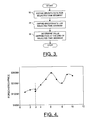
- FIG. 6 is a graph of a market potential distribution used during operation of the system, method and computer program product of one embodiment of the present invention.
- FIG. 7 is a schematic illustration of a market penetration distribution for a forecasted market used during operation of the system, method and computer program product of one embodiment of the present invention.
- FIG. 8 a is a schematic illustration of a price sensitivity distribution recast in reverse cumulative format used during operation of the system, method and computer program product for modeling demand according to one embodiment of the present invention
- FIG. 8 b is a schematic illustration of a price sensitivity distribution recast in cumulative format used during operation of the system, method and computer program product for modeling supply according to one embodiment of the present invention
- FIG. 9 a is a schematic illustration of a demand curve in a forecasted market for one time segment in a non-differentiated market, according to one embodiment of the present invention.
- FIG. 9 b is a schematic illustration of a supply curve in a forecasted market for one segment of a time period including a plurality of segments, according to one embodiment of the present invention.
- FIGS. 10 and 11 are flowcharts illustrating various steps in a method of modeling demand over a time segment in a differentiated market, in accordance with one embodiment of the present invention
- FIG. 12 a is a schematic illustration of a non-differentiated demand curve segmented into a plurality of market segments, in accordance with one embodiment of the present invention
- FIG. 12 b is a schematic illustration of a demand curve in a forecasted market for one time segment in a differentiated market and in a non-differentiated market, according to one embodiment of the present invention
- FIG. 13 a is a schematic illustration of a non-differentiated supply curve segmented into a plurality of market segments, in accordance with one embodiment of the present invention
- FIG. 13 b is a schematic illustration of a supply curve in a forecasted market for one time segment in a differentiated market, according to one embodiment of the present invention
- FIG. 14 is a flowchart illustrating various steps in a method of modeling demand over a time segment in an aggregate market including a plurality of component markets, in accordance with one embodiment of the present invention
- FIG. 15 is a schematic illustration of demand curves in three forecasted component markets, as well as in a corresponding aggregate market, according to one embodiment of the present invention.
- FIG. 16 is a schematic illustration of a demand curve in a forecasted market for three segments of a time period including a plurality of segments, according to one embodiment of the present invention.
- FIG. 17 is a schematic illustration of a cost curve used during operation of the system, method and computer program product of one aspect of the present invention in the context of a good purchased in a non-differentiated market;
- FIG. 18 is a schematic illustration comparing a demand curve with a cost curve, both modeled in accordance with embodiments of the present invention.
- FIG. 19 is a schematic illustration of a profitability curve according to one embodiment of the present invention.
- FIG. 20 is a schematic illustration of an optimum number of units of a good sold over a period of time, according to one embodiment of the present invention.
- FIG. 21 is a schematic illustration of a maximum profit for a good over a period of time, according to one embodiment of the present invention.
- FIG. 22 is a schematic illustration of the maximum profit for a good compared against the volatility (uncertainty) in the number of units of the good sold, according to one embodiment of the present invention.
- FIG. 23 is a schematic block diagram of the system of one embodiment of the present invention embodied by a computer.
- modeling uncertain future demand for a good generally begins by defining the period of time, as shown in block 10 .
- the period of time can then be divided into a number of different time segments.
- Each time segment begins at point in time t and ends at point in time t+1 (presuming the time segment is an integer divisor of T), and is defined by the beginning point in time t.
- the mean price and mean market size can be determined in any of a number of different manners such as, for example, based upon historical data, estimates or the like.
- Products can generally be categorized in either a non-differentiated market or a differentiated market.
- a non-differentiated market such as a commodity market
- goods are offered at one standard price, like $1.39 per pound or a listed price of $100M per item.
- a differentiated market the prices of the goods differ on a sale-by-sale or transaction-by-transaction basis because of differing perceived values. For example, the storeowner might discount the last three pounds of tomatoes at $1.00 per pound in order to clear end-of-the-day perishable stock.
- the listed price of $100M per item could be subjected to private negotiations resulting in a better match of the negotiated sale price to the marginal utility of the item to the consumer.
- the value of the distinguishing features are revealed and determined during private negotiations between a supplier and a consumer. Because the negotiated prices remain private, the process allows different amounts of goods to be sold at different prices. For example, wholesale lots of automobiles and aircraft are both goods that, due to differing features, can be sold at differing prices for differing quantities.
- Another type of differentiated market is one where there are sophisticated pricing systems that exploit small differences among buyer preferences, for example airplane seat, travel and concert seat reservation systems, and department store merchandise pricing coupled with membership discounting.
- the present invention provides systems, methods and computer program products for modeling demand for goods in a non-differentiated market as well as a differentiated market.
- the demand for a good in a non-differentiated market is generally a function of the price per unit of the good and the size of the market in terms of the total number of units of the good in the market, both of which differ depending upon the good.
- neither the price of the good nor the size of the market can be specified as each includes an amount of uncertainty.
- the demand is typically modeled based upon a distribution of the possible prices for which the good may be sold, and a distribution of the possible sizes of the market within which the good may be sold.
- modeling the uncertain future demand over the selected time segment includes assessing uncertainty in the price per unit of the good by determining how the price of the good affects whether customers will purchase the good, or in the case of modeling supply, how the price of the good affects whether manufacturers will produce the good.
- Uncertainty in the purchase price of each unit of the good is typically expressed in a price sensitivity distribution (e.g., lognormal distribution) of a unit purchase of the good at a predetermined price, as shown in block 20 .
- the price sensitivity distribution generally assigns a probability of a unit purchase to each respective price at which consumers would purchase the unit.
- the price sensitivity distribution can be developed from sparse data of real or hypothetical consumer purchases of at least one unit of the good at respective prices per unit developed according to any one of a number of different methods, such as from a number of historical sales, an expert's estimation, or a market survey.
- the distribution shown in FIG. 2 can be defined with as few as two points of price data, such as the price values 10% probability (only 10% of customers will purchase above a selected price) and 90% probability (90% of customers will purchase above a selected price). Additional data points, however, provide better accuracy of the price sensitivity distribution estimate.
- one method of determining a price sensitivity distribution or other value distribution includes defining the growth rate of the good for the selected time segment.
- the growth rate can be determined according to any of a number of different techniques, such as according to market forecasts.
- the growth rate can vary from time segment to time segment over the time period.
- the uncertainty can be determined according to any of a number of different techniques.
- the price sensitivity distribution (value distribution) can then be determined based upon the standard deviation in time for the selected time segment and the mean market price of the good for the time segment.
- the uncertainty is determined based upon a statistical analysis of average growth rate or a particular market, versus change in growth rate, resulting in a standard deviation calculation for uncertainty.
- risk and return need not have such a relationship.
- a linear relationship between risk and return is approximately reflective of the capital market relationship of risk and return, embodied in the well-known Capital Asset Pricing Model (CAPM) theory.
- CAPM Capital Asset Pricing Model
- risk and return may not have a linear relationship. For example, some goods may have a high projected return with corresponding low risk when compared to CAPM.
- the price sensitivity distribution (shown in FIG. 3 as a value distribution) can be determined based upon the standard deviation in time for the selected time segment and the mean price of the good for the time segment, as shown in block 36 .
- the mean price of the good for the selected time segment can be determined in one embodiment based upon the mean price of the good for the previous time segment, and the growth rate for the current, selected time segment. For example, the mean price of the good for the selected time segment can be determined as follows:
- ⁇ t ( 1 + GR t 100 ) ⁇ ⁇ t - 1 ( 1 )
- ⁇ t represents the mean price of the good for the current selected time segment
- ⁇ t-1 represents the mean value of the good at the immediately preceding time segment
- GR t represents the growth rate for the current selected time segment, where the growth rate is expressed in terms of a percentage.
- the standard deviation for the selected time segment can be determined in any of a number of different manners.
- t represents the current selected time segment
- ⁇ t represents the standard deviation for the current selected time segment.
- Future demand can be subject to a contingent activity, or event, which can impact the future demand (mean and uncertainty values) for subsequent time segments.
- price upon which demand is based
- the mean price of the good i.e., ⁇ t-1
- the contingent activity can itself be represented as a probability distribution.
- the contingent activity comprising a sudden change in the price of oil, or an unforeseen catastrophe can be represented by a price of the good if the contingent activity comes to fruition, and an associated probability of the contingent activity coming to fruition.
- any contingent activities to which the price of the good for the selected time segment are subject can be accounted for to adjust the growth rate, uncertainty, mean value and/or standard deviation accordingly.
- the price sensitivity distribution can be determined for the selected time segment by defining the respective price sensitivity distribution according to the respective mean value of the good and standard deviation.
- the price sensitivity distribution can be expressed according to any of a number of different probability distribution types such as normal, triangular or uniform. But because the economy typically functions in a lognormal fashion, in a typical embodiment the price sensitivity distribution is expressed as a lognormal probability distribution.
- a market potential distribution can similarly be determined before, after or during determination of the price sensitivity distribution, irrespective of exactly how the price sensitivity distribution is determined, as shown in block 22 .
- the demand can advantageously be modeled as a function of the size of the market within which the good is purchased to thereby account for uncertainty in the size of the market.
- Uncertainty in the size of the market is typically represented as a market potential that refers to the total number of units of the good consumers will purchase presuming all consumer requirements are met, including price.
- the market potential is typically expressed as a distribution of consumers purchasing a predetermined number of units of the good.
- the market potential distribution generally assigns a probability to each respective number of units of the good consumers will purchase presuming all consumer requirements are met.
- the market potential distribution for the selected time segment can be determined in any of a number of different manners but, in one typical embodiment, the market potential is determined in a manner similar to that of the price sensitivity distribution (see FIG. 3 ). More particularly, the growth rate and uncertainty in the market determined for the selected time segment can be determined in the same manner as that explained above (see blocks 32 and 34 ), and can be the same or different from that determined for the price sensitivity distribution.
- the market potential distribution (value distribution) can then be determined based upon the standard deviation in time for the selected time segment and the mean market size (number of units) of the good for the time segment.
- the mean market size (i.e., ⁇ t ) for the selected time segment is determined based upon the mean market size for the previous time segment (i.e., ⁇ t-1 ), and the growth rate for the current, selected time segment.
- the market potential distribution can then be determined based upon the standard deviation in time for the selected time segment and the mean market size for the time segment (see block 36 ).
- the market potential distribution can also be developed from sparse data from any one of a number of different sources, such as market studies or a myriad of other factors as known to those skilled in the art.
- the market potential distribution can be expressed according to any of a number of different probability distribution types such as normal, triangular or uniform but, like the market sensitivity distribution, the market potential distribution is typically expressed as a lognormal probability distribution.
- the demand for the good is modeled as a function of the size of the market within which the good is sold.
- a forecasted market of a predefined total number of units of the good is selected from the market potential distribution for the selected time segment.
- the number of units in the forecasted market is selected according to a method for randomly selecting a predefined number of units of the good, such as the Monte Carlo method.
- the Monte Carlo method is a method of randomly generating values for uncertain variables to simulate a model. The Monte Carlo method is applied to the market potential distribution to select the predefined number of units of the good in the forecasted market, as shown in block 24 of FIG. 2 .
- a market penetration distribution for the selected time segment can be determined based upon different numbers of units that represent corresponding percentages of the forecasted market, as shown in block 26 . For example, as shown in FIG. 7 , in a market size of 700 units of the good, a sale of 350 units would be associated with a market penetration of 50%. In an alternative market penetration distribution, represented as a dotted line in FIG.
- volume discounting may curve the market penetration distribution in a non-linear manner, such as in the case represented by the dotted line in FIG. 7 .
- the case represented by the straight line may represent a risk neutral market without volume discounting, such as a true commodity market.
- the dotted, curved line in FIG. 7 may represent a negative correlation between price and units sold in a contract (differentiated market).
- the demand for the selected time segment can be modeled based upon the price sensitivity distribution and the market penetration distribution for the selected time segment.
- the price sensitivity distribution is typically first recast in reverse cumulative format, as shown in FIG. 8 a . (see FIG. 2 , block 28 ).
- a reverse cumulative distribution depicts the number, proportion or percentage of values greater than or equal to a given value.
- the reverse cumulative of the price sensitivity distribution represents the distribution of a unit purchase of the good for at least a predetermined price, i.e., at or above a predetermined price.
- the price sensitivity distribution is typically first recast in cumulative format, as shown in FIG. 8 b .
- a cumulative distribution depicts the number, proportion or percentage of values less than or equal to a given value.
- the cumulative of the price sensitivity distribution represents the distribution of a unit manufactured when the market price for the good is at least a predetermined price, i.e., at or above a predetermined price.
- the demand represents the number of units consumers will purchase for at least a given price, i.e., at or above a given price.
- each probability percent of the reverse cumulative of the price sensitivity distribution is associated with a corresponding percentage of the forecasted market from the market penetration distribution.
- each of a plurality of different numbers of units of the good from the market penetration distribution are linked to a minimum price per unit from the reverse cumulative price sensitivity distribution having a probability percent equal to the market penetration percent for the respective number of units.
- the demand model can be thought of as a plurality of different numbers of units sold in the forecasted market, each number of units having a corresponding minimum price at which consumers will purchase the respective number of units. For example, a number of goods totaling 700 and having a market penetration of 100% is linked to a price per unit of approximately $77 million dollars having a probability percent of 100%. Thus, according to the demand model, 700 units of the good will sell for at least $77 million dollars.
- the demand model can be represented in any one of a number of manners but, in one embodiment, the demand model is represented as a demand curve by plotting different numbers of units sold in the forecasted market versus the minimum price consumers will pay per unit for the good, as shown in FIG. 9 a.
- the supply for the product in the forecasted market for the selected time segment can be modeled based upon the cumulative of the price sensitivity distribution and the market penetration distribution.
- the supply represents the number of units manufacturers will produce when the market price for the good is at least a given price, i.e., at or above a given price.
- each probability percent of the cumulative of the price sensitivity distribution is associated with a corresponding percentage of the forecasted market from the market penetration distribution.
- each of a plurality of different numbers of units of the good from the market penetration distribution are linked to a maximum price per unit from the cumulative price sensitivity distribution having a probability percent equal to the market penetration percent for the respective number of units.
- the supply model can be thought of as a plurality of different numbers of units produced in the forecasted market, each number of units having a corresponding maximum market price.
- the supply model can be represented in any one of a number of manners. In one embodiment, for example, the supply model is represented as a supply curve by plotting different numbers of units produced in the forecasted market versus the maximum market price of the good, as shown in FIG. 9 b.
- the steps in determining the reverse cumulative (or cumulative) of the price sensitivity distribution and the market penetration distribution can be accomplished in any order relative to one another without departing from the spirit and scope of the present invention.
- the price sensitivity distribution can be rewritten in reverse cumulative format before any or all of the steps in determining the market penetration distribution from the market potential distribution.
- the demand is typically modeled based upon a distribution of the possible prices for which the good may be sold, and a distribution of the possible sizes of the market within which the good may be sold and/or produced.
- the demand and/or supply for a good in a differentiated market over a period of time can be modeled based upon a price sensitivity distribution and a market potential distribution for each time segment, such as those explained above.
- non-differentiated markets differ from differentiated markets in that goods in non-differentiated markets are all sold and purchased for a uniform price, as opposed to differing prices based on individual units.
- the goods are sold according to contracts that each specify a predetermined number of units of the good at a predetermined price for each unit.
- modeling the demand for the good may further include assessing the uncertainty in the number of contracts in the market, as well as uncertainty in the predetermined number of units of the good in each contract and the predetermined price per unit at which each unit in each contract is purchased.
- demand in a differentiated market is estimated from demand in a non-differentiated market.
- demand in a differentiated market is modeled by first modeling demand in a non-differentiated market, as shown in block 38 .
- demand in the non-differentiated market can be modeled in any of a number of different manners
- demand in the non-differentiated market is modeled in the manner explained above with reference to FIGS. 2-9 .
- the non-differentiated demand model is integrated over the forecasted market to model or otherwise estimate demand for the good in a corresponding differentiated market.
- one method for integrating a non-differentiated demand model includes segmenting the forecasted market into a plurality of market segments.
- the forecasted market can then be segmented into a number of different market segments.
- Each market segment begins with unit u ⁇ 1% U and ends with unit u, and is defined by the ending unit u.
- the price per unit of the good over the selected market segment is calculated.
- the demand for the good in the forecasted market represents the number of units consumers may purchase for at least a given price.
- the price per unit of the selected market segment can be calculated by calculating the average the non-differentiated market price per unit of the good for the market segments up to, and including, the selected market segment, and associating the average with the selected market segment, as shown in blocks 46 and 48 .
- the associated price per unit can be calculated by averaging the non-differentiated market price per unit of the good for the market segments up to, and including, the respective market segment.
- demand for the good in the differentiated market can be modeled or otherwise estimated based upon the units u that define the market segments and the respective, associated prices per unit, as shown in block 52 .
- the differentiated demand model can be thought of as a plurality of different numbers of units sold in segments of the forecasted market, each number of units having a corresponding minimum price at which consumers will purchase the respective number of units.
- the differentiated demand model can be represented in any one of a number of manners but, in one embodiment, the differentiated demand model is represented as a demand curve by plotting the numbers of units sold in the forecasted market for the different market segments versus the minimum price consumers will pay per unit for the good, as shown in FIG. 12 b against a corresponding non-differentiated demand model.
- the supply for the product in a forecasted, differentiated market for the selected time segment can be modeled in a number of different manners, including that described in U.S. patent application Ser. No. 10/453,727.
- supply in a differentiated market can be modeled or otherwise estimated based upon a corresponding non-differentiated supply model.
- non-differentiated supply can be modeled, such as in the manner explained above.
- differentiated supply can be modeled by integrating the non-differentiated supply model.
- differentiated supply can be modeled by segmenting the forecasted market into a plurality of segments, as shown, for example, in FIG. 13 a for the non-differentiated supply model of FIG. 9 b . For each segment, then, an associated price per unit can be calculated by averaging the non-differentiated market price per unit of the good for the market including, and after, the respective market segment.
- the supply model can be thought of as the numbers of units produced in the forecasted market for each of a plurality of market segments, each market segment having a corresponding maximum market price.
- the supply model can be represented in any one of a number of manners.
- the supply model is represented as a supply curve by plotting the numbers of units produced in the forecasted market for the different market segments versus the maximum market price of the good, as shown in FIG. 13 b against a corresponding non-differentiated supply model.
- the steps in modeling demand/supply in a differentiated market can be accomplished in any of a number of different orders relative to one another, including the order explained above, without departing from the spirit and scope of the present invention.
- demand/supply in the differentiated market need not be modeled across the entire forecasted market.
- an aggregate traveler market may be formed when travelers from several connecting cities converge on a city-pair travel. More particularly, for example, travelers may have different origin and destination cities, but converge on a particular city-pair to complete their journey.
- a city-pair (A to B) market may comprise an aggregate market of up to four independent traveler route markets: “A to B,” “behind A to B,” “A to beyond B,” and “behind A to beyond B.”
- the automotive industry aggregate automobile markets for different types of automobiles, such as trucks, sedans, sport utility vehicles (SUVs) and the like, where the aggregate markets may be formed from component markets for different characteristics of the respective types of automobiles, such as for different makes, models or the like.
- an aggregate SUV market may be formed of component SUV markets, where all of the component markets generally include SUVs, but are distinct from one another in characteristics of the SUVs in the respective component market (e.g., size, performance, price, etc.).
- a SUV market may comprise an aggregate of smaller component SUV markets, such as a compact SUV market, mid-size SUV market, full-size SUV market, luxury SUV market and/or hybrid SUV market.
- each origin-destination market may have its own price (e.g., fare) and number of units of a good (e.g., travel tickets) relationship depending upon underlying economic dynamics. Travelers may pay differing prices for units of a good with differing origin and destination cities, but which include a common city-pair.
- demand is modeled for a good in an aggregate, differentiated market. It should be understood, however, that supply can be similarly modeled for a good in an aggregate, differentiated market without departing from the spirit and scope of the present invention. Further, it should be understood that demand and/or supply can equally be modeled for a good in an aggregate, non-differentiated market.
- a method of modeling demand in an aggregate market includes defining the component markets forming the aggregate market.
- Each component market can be defined in any of a number of different manners.
- each component market is defined by a price sensitivity distribution and, if so desired, a market potential distribution, where the distributions may be determined in a manner such as that explained above.
- demand for the good in each of the component markets is modeled as shown in block 56 .
- demand for the good in each of the component markets can be modeled in the manner explained above with respect to FIGS. 10 and 11 .
- the component-market demand models are combined to model demand for the good in the aggregate market, as shown in block 58 .
- the component-market demand models can be combined in a number of different manners.
- One technique referred to as the numerical method, models demand in the aggregate market utilizing the market segments and prices per unit of the good associated with those market segments for the component markets (calculated for the market segments during modeling of the component markets).
- demand in the aggregate market is modeled utilizing the market segments of the component markets and the distribution(s) defining the component markets.
- modeling demand in the aggregate market in accordance with the numerical method includes ranking the price per unit of each market segment across all of the component markets, such as in an ascending order from the lowest price per unit up, or in a descending order from the highest price per unit down.
- a cumulative number of units for each different price per unit can then be calculated.
- the cumulative number of units for each price can equal the cumulative number units sold for a price per unit equal to or greater than the respective price across all market segments of all of the component markets.
- the cumulative number of units for each price can equal the cumulative number units sold for a price per unit less than the respective price across all market segments of all of the component markets.
- the cumulative number of units associated with the highest price per unit would equal the number of units in each market segment having the highest price per unit.
- the cumulative number of units associated with the second highest price per unit would equal the number of units in each market segment having the second highest price per unit plus the number of units in each market segment having the highest price per unit.
- demand for the good in the aggregate market can be modeled based upon the price per unit of each of the segments and the cumulative number of units sold for a price per unit equal to or greater than the respective price per unit.
- the aggregate market demand model can be thought of as a plurality of different numbers of units sold in the forecasted, aggregate market, each number of units having a corresponding minimum price at which consumers will purchase the respective number of units. For examples of the demand of three component markets modeled relative to one another and relative to the corresponding aggregate market, see FIG. 15 .
- modeling demand in the aggregate market in accordance with the mathematical method includes calculating a mean price of the good and an associated standard deviation for the aggregate market.
- the mean and associated standard deviation for the aggregate market can be calculated in any of a number of different manners. Consider, for example, the case of differentiated markets, when demand for the good in each of the component markets is modeled in the manner explained above with respect to FIGS. 10 and 11 .
- the average price for each component market can then be weighted by multiplying the average price by the fraction of the number of units of the good in the component market to the number of units in the aggregate market.
- the mean can be calculated by summing the weighted average prices for the component markets.
- the associated standard deviation for the aggregate market can be calculated based upon weighted contributions of the component markets to the overall aggregate market.
- the calculation of the standard deviation can be similar to standard variance equations.
- the total number of units in the aggregate market, U can be calculated by summing the number of units in the component markets, U k .
- first and second sum values can be calculated as follows:
- MultiMarketStdDev ( U ⁇ Sum ⁇ ⁇ 1 ) - Sum ⁇ ⁇ 2 2 U 2 - U ( 6 )
- a price sensitivity distribution of a unit purchase of the good in the aggregate market can be determined for the selected time segment by defining the respective price sensitivity distribution according to the respective mean value of the good and standard deviation, such as in the same manner explained above and in the aforementioned '727 application (see FIG. 5 ).
- a market penetration for the aggregate market can be determined from the aggregate number of units of the good, U. More particularly, for example, a market penetration for the aggregate market can be determined based upon the different numbers of units that represent corresponding percentages of the forecasted market, as also explained above and in the '727 application (see FIG. 7 ). Then, once the price sensitivity and market penetration distributions have been determined, the demand for the good in the aggregate market can be modeled based upon the price sensitivity distribution and the market penetration distribution for the selected time segment. To combine the price sensitivity distribution and the market penetration distribution, the price sensitivity distribution can be recast in reverse cumulative format (see FIG. 8 a ). Demand for the good in the aggregate market can then be modeled based upon the reverse cumulative of the price sensitivity distribution and the market penetration distribution, such as in the same manner explained above and in the '727 application (see FIG. 9 a ).
- the “market” described below may comprise a non-differentiated or differentiated market, which may represent a single market, component market or aggregate market. For each time segment of the time period in a non-differentiated market, for example, a price sensitivity distribution and market potential distribution can be determined (see blocks 20 and 22 ).
- a forecasted market size can be selected, with a market penetration distribution determined based upon the forecasted market (see blocks 24 and 26 ).
- the price sensitivity distribution can be rewritten into a reverse cumulative distribution (see block 28 ), which can thereafter be used with the market penetration distribution to model demand for the respective time segment.
- the demand model for the different segments can be represented in any one of a number of manners but, in one embodiment, the demand models are represented as demand curves by plotting different numbers of units sold in the forecasted market for each segment versus the minimum price consumers will pay per unit for the good, as shown with respect to three segments (i.e., years 1, 10 and 19) in FIG. 16 .
- modeling the demand for the good can be used with a cost model to model profitability for the good in the forecasted market for each time segment.
- the profitability model can be used to determine conclusions regarding the good over the period of time, such as the optimum price per unit and the number of units sold for each time segment.
- the conclusions for the segments of the time period can then be used, such as by the manufacturer, to facilitate an understanding of how uncertainty in the price of the good and number of units in the market affect demand for the good over time.
- the manufacturer can be in a better position to select a price at which to sell each unit of the good, as well as a number of units of the good to produce.
- the profitability of the good over the time segments of the time period can be modeled thereby facilitating an understanding of how uncertainty in demand for the good, as well as uncertainty in cost of producing the good, can affect profitability over time.
- the demand model differs depending on whether the goods are in a non-differentiated market or a differentiated market
- the profitability of the good also differs depending on the type of market.
- the present invention provides systems, methods and computer program products for modeling the profitability of a good over time in both non-differentiated markets as well as differentiated markets.
- Modeling the profitability of a good over segments of a time period in a non-differentiated market generally includes modeling the demand for the good over those segments, such as according to embodiments of the present invention as described above with reference to FIGS. 1-9 .
- the cost of producing the good is also modeled over the segments of the time period.
- the cost model for each time segment can be based on the average cost per unit to produce the good and the number of units produced, or sold.
- the cost model for a time segment accounts for uncertainty in the size of the market, just as does the demand model for that time segment.
- the cost of producing the good can be modeled in any one of a number of manners, the cost preferably considers the effect of the number of units produced, or sold, on the cost to produce each unit of the good. Costs associated with producing a good in many markets tend to decline as the manufacturer gains experience with that production.
- the cost to produce each unit of the good is typically more than the expected cost of producing each unit for the first units produced. And as the number of units produced increases, the manufacturer typically gains experience that drives the cost to produce each unit down to and below the expected cost, and thereafter eventually leveling to an optimum cost of producing each unit.
- the change in the cost to produce each unit can generally be considered to be attributable to a “learning curve” experienced by the manufacturer in manufacturing the good.
- a cost model accounting for a learning curve can be represented in any one of a number of different manners but, in one embodiment, the cost model is represented as a reverse cumulative cost curve by plotting the different costs per unit versus the cumulative number of units produced for the respective cost per unit, as shown in FIG. 17 .
- the cost model is represented as a reverse cumulative cost curve by plotting the different costs per unit versus the cumulative number of units produced for the respective cost per unit, as shown in FIG. 17 .
- FIG. 17 As an example of one method by which the cost to produce each unit of a good in a non-differentiated market can be modeled, see U.S. patent application Ser. No. 10/453,779, entitled: Systems, Methods and Computer Program Products for Determining A Learning Curve Value and Modeling Associated Profitability and Costs of A Good, filed Jun. 3, 2003, the contents of which are hereby incorporated by reference in its entirety.
- the profitability for the good in the forecasted market for the respective time segment can be modeled.
- the profitability for a time segment can be represented as the result of subtracting the cost per unit from the price per unit and multiplying the difference by the number of units sold for the corresponding fraction of the forecasted market.
- graphically, as shown in FIG. 18 with respect to a given time segment by simultaneously plotting the demand curve and the cost curve for the forecasted market, the profitability for the respective time segment can be seen as directly related to the distance between the two curves.
- the profitability model for the respective time segment can be represented in any one of a number of different manners. In one embodiment, shown in FIG. 19 , the profitability model for a given time segment can be represented as a profitability curve by plotting the number of units that must be sold to achieve at least a given profit.
- conclusions regarding the forecasted market of the respective time segment can be drawn from collectively modeling the demand, cost and profitability for the forecasted market of the respective time segment.
- the maximum profit for the good in the forecasted market of the respective time segment can be seen as the point where the price exceeds the cost by the greatest amount.
- the maximum profit the optimum price for each unit of the good and the optimum number of units sold in the forecasted market (i.e., fraction of the number of goods in the market), as well as the corresponding cost associated with the optimum price and number of units sold, in the forecasted market of the respective time segment can be determined.
- the maximum profit margin for the forecasted market of the respective time segment can be determined by dividing the difference between the optimum price and associated cost by the optimum price, and thereafter recorded. Further, the price per unit and number of units at which the forecasted market clears can be determined from the point where the profitability is zero (or the point where the demand model intersects the cost model).
- the profitability for the good in a forecasted market can similarly be modeled for each of the time segments t of the time period T, with conclusions drawn from the respective demand, cost and profitability models for the respective time segments. Those conclusions can then be plotted to develop or otherwise create a business case for the good over time.
- the business case can receive the optimum number of units for each time segment, and plot the optimum number of units over the time period, as shown in FIG. 20 .
- the business case can receive the maximum forecasted profit (e.g., gross profit) for each time segment, and plot the maximum profit over the time period, as shown in FIG. 21 .
- the business case can receive the maximum forecasted profit for each time segment, and plot the maximum profit against the volatility (uncertainty) in the number of units of the good sold (see block 22 of FIG. 2 with respect to determining the market potential distribution), as shown in FIG. 22 . From the illustrated scatter plot, then, a best fit curve can be formed from the points of maximum profit and associated uncertainty in the number of units of the good to illustrate the consistency, or lack thereof, in profitability of the good in an uncertain market.
- modeling the profitability can proceed in a manner similar to that explained above with respect to modeling the profitability in non-differentiated markets.
- the demand for the good and cost of producing the good for each time segment can be modeled in a manner similar to that explained above and in U.S. patent application Ser. No. 10/453,727.
- Profitability in the differentiated market for each time segment can then be represented in a manner similar to the non-differentiated market.
- conclusions regarding the forecasted market for each time segment can be drawn from collectively modeling the demand, cost (or lowest cost value) and profitability for the forecasted market in the respective time segments.
- the profitability model actually demonstrates a negative profitability, or a loss for sales of the good, as shown in FIG. 19 .
- Contingent claims oftentimes come in the form of a call in which the manufacturer has an option to invest an amount of money, or additional amounts of money, in order to start producing or continue producing the good.
- the manufacturer will likely decline to invest the money, or additional money, and thereby forego exercise of the call and will therefore decline to produce the good or terminate production of the good.
- the manufacturer will likely make the necessary investment in order to begin or continue production of the good.
- the manufacturer can avoid overpaying for production of the good as a result of an overvaluation of the contingent claim.
- the manufacturer can identify goods in which the value of the contingent claim has been undervalued and can give strong consideration to investing in the production of these goods since they likely represent worthwhile investment opportunities.
- the systems, methods and computer program products of the present invention can facilitate determining the value of the good and, in particular, the contingent claim at the present time.
- the systems, methods and computer program products of the present invention therefore are capable of modeling uncertain future demand, supply and associated profitability of a good over a period of time based on sparse historical data or estimates regarding price and quantity of the good.
- embodiments of the present invention are capable of modeling uncertain future demand, supply and, thus the profitability as a function of the size of the market within which the good is sold more adequately than conventional methods of modeling the demand.
- embodiments of the present invention are capable of modeling uncertain future demand, supply and associated profitability for each segment of the time period while better accounting for how changing the price of the good changes the number of units of the good purchased.
- embodiments of the present invention are capable of modeling uncertain future demand, supply and associated profitability over time to thereby facilitate an understanding of how uncertainty in a market over time affects demand, supply and profitability.
- Such an understanding can be advantageous to those associated with the manufacture, sale and purchase of the good, such as in the context of commercial transactions.
- Programs for the future sale of goods inherently have associated uncertainty, particularly as it relates to the market for the goods, typically defined by the number of good purchased and the price at which each unit of the good is purchased.
- demand, supply and associated profitability of a good can be modeled in a manner such that a manufacturer can be in a better position to not only decide whether to bring a good to market, but to also select a price at which to sell each unit of the good, as well as a number of units of the good to produce.
- the system of embodiments of the present invention is typically embodied by a processing element and an associated memory device, both of which are commonly comprised by a computer 60 or the like.
- the method of embodiments of the present invention can be performed by the processing element manipulating data stored by the memory device with any one of a number of commercially available computer software programs.
- the method can be performed with data that is capable of being manipulated and/or presented in spreadsheet form.
- the method can be performed by the processing element manipulating data stored by the memory device with Excel, a spreadsheet software program distributed by the Microsoft Corporation of Redmond, Wash., including Crystal Ball, a Monte Carlo simulation software program distributed by Decisioneering, Inc. of Denver, Colo.
- the computer can include a display 62 for presenting information relative to performing embodiments of the method of the present invention, including the various distributions, models and/or conclusions as determined according to embodiments of the present invention.
- the computer can further include a printer 64 .
- the computer 60 can include a means for locally or remotely transferring the information relative to performing embodiments of the method of the present invention.
- the computer can include a facsimile machine 66 for transmitting information to other facsimile machines, computers or the like.
- the computer can include a modem 68 to transfer information to other computers or the like.
- the computer can include an interface (not shown) to a network, such as a local area network (LAN), and/or a wide area network (WAN).
- LAN local area network
- WAN wide area network
- the computer can include an Ethernet Personal Computer Memory Card International Association (PCMCIA) card configured to transmit and receive information to and from a LAN, WAN or the like.
- PCMCIA Personal Computer Memory Card International Association
- the methods according to embodiments of the present invention may be embodied in a software or data module, component, portfolio or the like, that can be manipulated or otherwise operated within a spreadsheet software program such as Excel.
- a technique may be advantageous in a number of different contexts, such as in the context of financial modeling and analysis. Modules, components and/or portfolio that perform various financial modeling functions can be combined to gain a more complete understanding of a financial context. A brief description of such a technique as such may be applied to the present invention will now be described below.
- data capable of being manipulated to perform at least a portion of the methods of the present invention can be embodied in a module, which can thereafter be linked or otherwise associated with other portions of the methods of the present invention embodied in other modules so as to formulate a component. Then, if so desired, the component can be linked or otherwise associated with other components capable of performing other related methods to thereby form a portfolio.
- methods of modeling future demand according to embodiments of the present invention can be embodied in one module while methods of modeling cost according to embodiments of the present invention can be embodied in another module.
- the two modules can then be linked or otherwise associated with one another to formulate a component capable of generating a business case capable of modeling the profitability of the good based upon the future demand and cost. Then, if so desired, the component for generating the business case can be linked or otherwise associated with another component to perform another function.
- the system of the present invention generally operates under control of a computer program product.
- the computer program product for performing the methods of embodiments of the present invention includes a computer-readable storage medium, such as the non-volatile storage medium, and computer-readable program code portions, such as a series of computer instructions, embodied in the computer-readable storage medium.
- the computer-readable program code portions may include separate executable portions for performing distinct functions to accomplish methods of embodiments of the present invention.
- one or more of the computer-readable program portions may include one or more executable portions for performing more than one function to thereby accomplish methods of embodiments of the present invention.
- FIGS. 1 and 2 are a flowchart of methods, systems and program products according to the invention. It will be understood that each block or step of the flowchart, and combinations of blocks in the flowchart, can be implemented by computer program instructions. These computer program instructions may be loaded onto a computer or other programmable apparatus to produce a machine, such that the instructions which execute on the computer or other programmable apparatus create means for implementing the functions specified in the flowchart block(s) or step(s). These computer program instructions may also be stored in a computer-readable memory that can direct a computer or other programmable apparatus to function in a particular manner, such that the instructions stored in the computer-readable memory produce an article of manufacture including instruction means which implement the function specified in the flowchart block(s) or step(s).
- the computer program instructions may also be loaded onto a computer or other programmable apparatus to cause a series of operational steps to be performed on the computer or other programmable apparatus to produce a computer implemented process such that the instructions which execute on the computer or other programmable apparatus provide steps for implementing the functions specified in the flowchart block(s) or step(s).
- blocks or steps of the flowchart support combinations of means for performing the specified functions, combinations of steps for performing the specified functions and program instruction means for performing the specified functions. It will also be understood that each block or step of the flowchart, and combinations of blocks or steps in the flowchart, can be implemented by special purpose hardware-based computer systems which perform the specified functions or steps, or combinations of special purpose hardware and computer instructions.
Abstract
Description
Risk(Return)=4×(Return−5)
where return and risk are expressed as percentages. For a further description of modeling risk as a function of returns, see U.S. patent application Ser. No. 10/453,395, entitled: Systems, Methods and Computer Program Products for Modeling A Monetary Measure for A Good Based Upon Technology Maturity Levels, filed Jun. 3, 2003, the contents of which is incorporated by reference in its entirety. For an example of the uncertainty (risk) associated with various growth rates (returns), as such may have been determined according to the above, see Table 1.
| TABLE 1 | |||
| Growth Rate | Uncertainty | ||
| 10.0% | 20% | ||
| 12.5% | 30% | ||
| 15.0% | 40% | ||
| 17.5% | 50% | ||
| 20.0% | 60% | ||
| 22.5% | 70% | ||
| 25.0% | 80% | ||
| 27.5% | 90% | ||
| 30.0% | 100% | ||
In equation (1), μt represents the mean price of the good for the current selected time segment, μt-1 represents the mean value of the good at the immediately preceding time segment, and GRt represents the growth rate for the current selected time segment, where the growth rate is expressed in terms of a percentage.
σt=μt×√{square root over (e σ
In equation (2), t represents the current selected time segment, and σt represents the standard deviation for the current selected time segment. Also in equation (2), σavgt represents a running average of the uncertainty values from t=1 to the current selected time segment t, and can be determined, for example, as follows:
where Ui represents the uncertainty for the ith time segment, and i=1, 2, . . . t. For an example of the values of the growth rate, mean price of the good, uncertainty and standard deviation for each time segment in a period of 30 years, where each time segment represents one year, see Table 2 below.
| TABLE 2 | ||||
| Growth Rate | ||||
| Time (t) | (GRt) | Mean (μt) | Uncertainty(Ui) | Std. Dev. (σt) |
| 0 | — | $500 | — | — |
| 1 | 20% | $600 | 60% | $395 |
| 2 | 20% | $720 | 60% | $739 |
| 3 | 20% | $864 | 60% | $1,205 |
| 4 | 20% | $1,037 | 60% | $1,861 |
| 5 | 20% | $1,244 | 60% | $2,796 |
| 6 | 20% | $1,493 | 60% | $4,135 |
| 7 | 20% | $1,792 | 60% | $6,057 |
| 8 | 20% | $2,150 | 60% | $8,816 |
| 9 | 20% | $2,580 | 60% | $12,779 |
| 10 | 20% | $3,096 | 60% | $18,471 |
| 11 | 18% | $3,653 | 52% | $25,034 |
| 12 | 16% | $4,238 | 44% | $32,051 |
| 13 | 14% | $4,831 | 36% | $39,026 |
| 14 | 12% | $5,411 | 28% | $45,483 |
| 15 | 10% | $5,952 | 20% | $51,056 |
| 16 | 8% | $6,428 | 20% | $56,269 |
| 17 | 6% | $6,813 | 20% | $60,866 |
| 18 | 4% | $7,086 | 20% | $64,595 |
| 19 | 2% | $7,228 | 20% | $67,234 |
| 20 | 0% | $7,228 | 20% | $68,608 |
| 21 | −2% | $7,083 | 20% | $68,609 |
| 22 | −4% | $6,800 | 20% | $67,209 |
| 23 | −6% | $6,392 | 20% | $64,466 |
| 24 | −8% | $5,880 | 20% | $60,518 |
| 25 | −10% | $5,292 | 20% | $55,577 |
| 26 | −12% | $4,657 | 28% | $50,880 |
| 27 | −14% | $4,005 | 36% | $46,710 |
| 28 | −16% | $3,364 | 44% | $43,253 |
| 29 | −18% | $2,759 | 52% | $40,631 |
| 30 | −20% | $2,207 | 60% | $38,942 |
where Priceu
Claims (15)
Priority Applications (1)
| Application Number | Priority Date | Filing Date | Title |
|---|---|---|---|
| US11/190,684 US7739166B2 (en) | 2003-06-03 | 2005-07-27 | Systems, methods and computer program products for modeling demand, supply and associated profitability of a good in a differentiated market |
Applications Claiming Priority (3)
| Application Number | Priority Date | Filing Date | Title |
|---|---|---|---|
| US10/453,727 US7627495B2 (en) | 2003-06-03 | 2003-06-03 | Systems, methods and computer program products for modeling demand, supply and associated profitability of a good |
| US10/453,396 US20040249642A1 (en) | 2003-06-03 | 2003-06-03 | Systems, methods and computer program products for modeling uncertain future benefits |
| US11/190,684 US7739166B2 (en) | 2003-06-03 | 2005-07-27 | Systems, methods and computer program products for modeling demand, supply and associated profitability of a good in a differentiated market |
Related Parent Applications (2)
| Application Number | Title | Priority Date | Filing Date |
|---|---|---|---|
| US10/453,396 Continuation-In-Part US20040249642A1 (en) | 2001-07-10 | 2003-06-03 | Systems, methods and computer program products for modeling uncertain future benefits |
| US10/453,727 Continuation-In-Part US7627495B2 (en) | 2003-06-03 | 2003-06-03 | Systems, methods and computer program products for modeling demand, supply and associated profitability of a good |
Publications (2)
| Publication Number | Publication Date |
|---|---|
| US20050262012A1 US20050262012A1 (en) | 2005-11-24 |
| US7739166B2 true US7739166B2 (en) | 2010-06-15 |
Family
ID=35376394
Family Applications (1)
| Application Number | Title | Priority Date | Filing Date |
|---|---|---|---|
| US11/190,684 Expired - Fee Related US7739166B2 (en) | 2003-06-03 | 2005-07-27 | Systems, methods and computer program products for modeling demand, supply and associated profitability of a good in a differentiated market |
Country Status (1)
| Country | Link |
|---|---|
| US (1) | US7739166B2 (en) |
Cited By (2)
| Publication number | Priority date | Publication date | Assignee | Title |
|---|---|---|---|---|
| US20100106555A1 (en) * | 2008-10-23 | 2010-04-29 | Sap Ag | System and Method for Hierarchical Weighting of Model Parameters |
| US8768812B2 (en) | 2011-05-02 | 2014-07-01 | The Boeing Company | System, method and computer-readable storage medium for valuing a performance option |
Families Citing this family (6)
| Publication number | Priority date | Publication date | Assignee | Title |
|---|---|---|---|---|
| US7379923B2 (en) * | 2003-11-06 | 2008-05-27 | International Business Machines Corporation | Benchmarking of computer and network support services |
| US8255269B1 (en) * | 2006-11-11 | 2012-08-28 | Samir Aued | Data processing method for maximization of present and future supply and/or demand objectives |
| US20100138273A1 (en) * | 2008-12-01 | 2010-06-03 | Arash Bateni | Repeatability index to enhance seasonal product forecasting |
| US20110178839A1 (en) * | 2010-01-20 | 2011-07-21 | Adra Hosni I | Method and system for evaluating a consumer product based on web-searchable criteria |
| US20190147462A1 (en) * | 2017-11-10 | 2019-05-16 | Target Brands, Inc. | Hybrid demand model for promotion planning |
| US11682030B2 (en) * | 2018-11-09 | 2023-06-20 | Ebay Inc. | Automatic listing of items based on user specified parameters |
Citations (64)
| Publication number | Priority date | Publication date | Assignee | Title |
|---|---|---|---|---|
| US5377095A (en) | 1991-07-12 | 1994-12-27 | Hitachi, Ltd. | Merchandise analysis system with sales data table and various functions for predicting the sale by item |
| US5692233A (en) | 1992-05-28 | 1997-11-25 | Financial Engineering Associates, Inc. | Integrated system and method for analyzing derivative securities |
| US5710578A (en) | 1987-12-09 | 1998-01-20 | International Business Machines Corporation | Computer program product for utilizing fast polygon fill routines in a graphics display system |
| US5960407A (en) | 1996-10-08 | 1999-09-28 | Vivona; Robert G. | Automated market price analysis system |
| US6061662A (en) | 1997-08-15 | 2000-05-09 | Options Technology Company, Inc. | Simulation method and system for the valuation of derivative financial instruments |
| US6078901A (en) | 1997-04-03 | 2000-06-20 | Ching; Hugh | Quantitative supply and demand model based on infinite spreadsheet |
| US6078893A (en) | 1998-05-21 | 2000-06-20 | Khimetrics, Inc. | Method for stabilized tuning of demand models |
| US6157918A (en) | 1995-07-07 | 2000-12-05 | Swychco Infrastructure Services Pty Ltd. | Methods and apparatus relating to the formulation and trading of investment contracts |
| US6205431B1 (en) | 1998-10-29 | 2001-03-20 | Smart Software, Inc. | System and method for forecasting intermittent demand |
| US20010041996A1 (en) | 1997-01-06 | 2001-11-15 | Eder Jeffrey Scott | Method of and system for valuing elements of a business enterprise |
| US6321212B1 (en) | 1999-07-21 | 2001-11-20 | Longitude, Inc. | Financial products having a demand-based, adjustable return, and trading exchange therefor |
| US6321205B1 (en) | 1995-10-03 | 2001-11-20 | Value Miner, Inc. | Method of and system for modeling and analyzing business improvement programs |
| JP2001357189A (en) | 2000-06-14 | 2001-12-26 | Nomura Securities Co Ltd | Decision-making support device for market participation |
| US20020010667A1 (en) | 1997-08-21 | 2002-01-24 | Elaine Kant | System and method for financial instrument modeling and using monte carlo simulation |
| EP1178416A1 (en) | 1999-08-27 | 2002-02-06 | Kabushiki Kaisha Toshiba | System for evaluating price risk of financial product or its financial derivative, dealing system, and recorded medium |
| US6381586B1 (en) | 1998-12-10 | 2002-04-30 | International Business Machines Corporation | Pricing of options using importance sampling and stratification/ Quasi-Monte Carlo |
| US6393406B1 (en) | 1995-10-03 | 2002-05-21 | Value Mines, Inc. | Method of and system for valving elements of a business enterprise |
| US20020116348A1 (en) * | 2000-05-19 | 2002-08-22 | Phillips Robert L. | Dynamic pricing system |
| US20020143604A1 (en) | 2001-02-02 | 2002-10-03 | Wisconsin Alumni Research Foundation | Method for forecasting the effects of trade policies and supply and demand conditions on the world dairy sector |
| US20030014337A1 (en) | 2001-07-10 | 2003-01-16 | Mathews Scott H. | Systems, methods and computer program products for performing a generalized contingent claim valuation |
| US20030033191A1 (en) | 2000-06-15 | 2003-02-13 | Xis Incorporated | Method and apparatus for a product lifecycle management process |
| US20030115128A1 (en) * | 1999-07-21 | 2003-06-19 | Jeffrey Lange | Derivatives having demand-based, adjustable returns, and trading exchange therefor |
| US20030144897A1 (en) | 2002-01-30 | 2003-07-31 | Burruss James W. | Finite life cycle demand forecasting |
| US6629082B1 (en) | 1999-06-15 | 2003-09-30 | W.R. Hambrecht & Co. | Auction system and method for pricing and allocation during capital formation |
| US20030236738A1 (en) * | 1999-07-21 | 2003-12-25 | Jeffrey Lange | Replicated derivatives having demand-based, adjustable returns, and trading exchange therefor |
| US20040068455A1 (en) | 2002-10-03 | 2004-04-08 | Jacobus Greg C. | Graphical user interface for procurement risk management system |
| US20040098327A1 (en) | 2002-11-14 | 2004-05-20 | Seaman David A. | Contingent convertible securities instrument and method of providing, trading and using the same |
| US20040128221A1 (en) | 2002-12-09 | 2004-07-01 | Pandher Gurupdesh S. | Option valuation method and apparatus |
| US6810332B2 (en) | 2003-01-31 | 2004-10-26 | Chevron U.S.A. Inc. | Method for computing complexity, confidence and technical maturity indices for reservoir evaluations |
| US20040249642A1 (en) | 2003-06-03 | 2004-12-09 | The Boeing Company | Systems, methods and computer program products for modeling uncertain future benefits |
| US6853952B2 (en) | 2003-05-13 | 2005-02-08 | Pa Knowledge Limited | Method and systems of enhancing the effectiveness and success of research and development |
| US20050102213A1 (en) | 2003-11-07 | 2005-05-12 | Serkan Savasoglu | Systems and methods for accreting remarketable convertible securities |
| US20050125318A1 (en) | 2003-11-29 | 2005-06-09 | Joel Jameson | Methods and systems for accurately representing corporate financial results in light of equity-based compensation and contingent transactions |
| US6910017B1 (en) | 1999-03-05 | 2005-06-21 | Profitlogic, Inc. | Inventory and price decision support |
| US6963854B1 (en) | 1999-03-05 | 2005-11-08 | Manugistics, Inc. | Target pricing system |
| US7085734B2 (en) | 2001-07-06 | 2006-08-01 | Grant D Graeme | Price decision support |
| US7110956B1 (en) | 1996-05-28 | 2006-09-19 | Texas Instruments Incorporated | Capability predictor |
| US20060253355A1 (en) | 2005-05-04 | 2006-11-09 | Chicago Board Options Exchange | System and method for creating and trading a digital derivative investment instrument |
| US20070011065A1 (en) | 2005-07-07 | 2007-01-11 | Santosh Sreenivasan | Method and system for pre-funding with merger call flexibility |
| US20070022031A1 (en) | 2005-07-19 | 2007-01-25 | Real Estate Equity Exchange Cayman, Inc. | Transfering financial interest |
| US20070050282A1 (en) | 2005-08-25 | 2007-03-01 | Sas Institute Inc. | Financial risk mitigation optimization systems and methods |
| US7197474B1 (en) | 2001-07-12 | 2007-03-27 | Vignette Corporation | Method of modeling product demand subject to a large number of interactions |
| US20070106576A1 (en) | 2005-10-21 | 2007-05-10 | Searete Llc, A Limited Liability Corporation Of The State Of Delaware | Disposition of component virtual property rights |
| US20070112661A1 (en) | 2001-07-10 | 2007-05-17 | The Boeing Company | System, method and computer program product for determining a minimum asset value for exercising a contingent claim of an option |
| US20070150392A1 (en) | 2001-07-10 | 2007-06-28 | The Boeing Company | System, method and computer program product for performing a contingent claim valuation of a combination option |
| US20070150395A1 (en) | 2001-07-10 | 2007-06-28 | The Boeing Company | System, method and computer program product for determining a minimum asset value for exercising a contingent claim of an option |
| US20070150391A1 (en) | 2001-07-10 | 2007-06-28 | The Boeing Company | System, method and computer program product for performing a contingent claim valuation of an early-launch option |
| US20070150394A1 (en) | 2001-07-10 | 2007-06-28 | The Boeing Company | System, method and computer program product for determining a minimum asset value for exercising a contingent claim of an option |
| US20070150393A1 (en) | 2001-07-10 | 2007-06-28 | The Boeing Company | System, method and computer program product for determining a minimum asset value for exercising a contingent claim of an option |
| US20070150390A1 (en) | 2001-07-10 | 2007-06-28 | The Boeing Company | System, method and computer program product for performing a contingent claim valuation of a multi-stage option |
| US20070162376A1 (en) | 2001-07-10 | 2007-07-12 | The Boeing Company | System, method and computer program product for determining a minimum asset value for exercising a contingent claim of an option |
| US20070299753A1 (en) | 2003-12-19 | 2007-12-27 | Michael Averbuch | Participatory equity appreciation contract ("PEAC") |
| US7315842B1 (en) | 2001-08-06 | 2008-01-01 | Wang Shaun S | Computer system and method for pricing financial and insurance risks with historically-known or computer-generated probability distributions |
| US20080015871A1 (en) | 2002-04-18 | 2008-01-17 | Jeff Scott Eder | Varr system |
| US7349878B1 (en) | 1996-08-16 | 2008-03-25 | Options Technology Company, Inc. | Simulation method and system for the valuation of derivative financial instruments |
| US20080109341A1 (en) | 2005-11-03 | 2008-05-08 | Genworth Financial Inc. | System and Method For Providing A Deferred Premium Annuity |
| US7398221B1 (en) | 2001-03-30 | 2008-07-08 | Rapt, Inc. | Method and apparatus for component plan analysis under uncertainty |
| US20080167984A1 (en) | 2007-01-05 | 2008-07-10 | Matthew Courey | Zero recovery credit default swap indices |
| US20080208678A1 (en) | 2000-10-06 | 2008-08-28 | Walser Joachim P | Generating an Optimized Price Schedule for a Product |
| US20080288394A1 (en) | 2000-10-17 | 2008-11-20 | Jeffrey Scott Eder | Risk management system |
| US20090030822A1 (en) | 2007-03-12 | 2009-01-29 | Jpmorgan Chase Bank, N.A. | System and Method for Contingent Equity Return Forward to Hedge Foreign Exchange Risk in Investments Having Varying Exit Parameters |
| US20090043683A1 (en) | 2005-02-04 | 2009-02-12 | Searete Llc, A Limited Liability Corporation Of The State Of Delaware | Virtual world reversion rights |
| US20090043604A1 (en) | 2005-02-04 | 2009-02-12 | Searette Llc, A Limited Liability Corporation Of The State Of Delaware | Disposition of component virtual property rights |
| US7574394B2 (en) | 2005-02-16 | 2009-08-11 | Sri, Inc. | Systems and methods for implementing the structuring, pricing, quotation, and trading of financial instruments |
Family Cites Families (1)
| Publication number | Priority date | Publication date | Assignee | Title |
|---|---|---|---|---|
| US7801804B2 (en) * | 2007-10-10 | 2010-09-21 | The Board Of Trustees Of The Leland Stanford Junior University | Convex parimutuel contingent claim market mechanism |
-
2005
- 2005-07-27 US US11/190,684 patent/US7739166B2/en not_active Expired - Fee Related
Patent Citations (69)
| Publication number | Priority date | Publication date | Assignee | Title |
|---|---|---|---|---|
| US5710578A (en) | 1987-12-09 | 1998-01-20 | International Business Machines Corporation | Computer program product for utilizing fast polygon fill routines in a graphics display system |
| US5377095A (en) | 1991-07-12 | 1994-12-27 | Hitachi, Ltd. | Merchandise analysis system with sales data table and various functions for predicting the sale by item |
| US5692233A (en) | 1992-05-28 | 1997-11-25 | Financial Engineering Associates, Inc. | Integrated system and method for analyzing derivative securities |
| US6157918A (en) | 1995-07-07 | 2000-12-05 | Swychco Infrastructure Services Pty Ltd. | Methods and apparatus relating to the formulation and trading of investment contracts |
| US6393406B1 (en) | 1995-10-03 | 2002-05-21 | Value Mines, Inc. | Method of and system for valving elements of a business enterprise |
| US6321205B1 (en) | 1995-10-03 | 2001-11-20 | Value Miner, Inc. | Method of and system for modeling and analyzing business improvement programs |
| US7110956B1 (en) | 1996-05-28 | 2006-09-19 | Texas Instruments Incorporated | Capability predictor |
| US7349878B1 (en) | 1996-08-16 | 2008-03-25 | Options Technology Company, Inc. | Simulation method and system for the valuation of derivative financial instruments |
| US5960407A (en) | 1996-10-08 | 1999-09-28 | Vivona; Robert G. | Automated market price analysis system |
| US20010041996A1 (en) | 1997-01-06 | 2001-11-15 | Eder Jeffrey Scott | Method of and system for valuing elements of a business enterprise |
| US6078901A (en) | 1997-04-03 | 2000-06-20 | Ching; Hugh | Quantitative supply and demand model based on infinite spreadsheet |
| US6061662A (en) | 1997-08-15 | 2000-05-09 | Options Technology Company, Inc. | Simulation method and system for the valuation of derivative financial instruments |
| US20020010667A1 (en) | 1997-08-21 | 2002-01-24 | Elaine Kant | System and method for financial instrument modeling and using monte carlo simulation |
| US6078893A (en) | 1998-05-21 | 2000-06-20 | Khimetrics, Inc. | Method for stabilized tuning of demand models |
| US6205431B1 (en) | 1998-10-29 | 2001-03-20 | Smart Software, Inc. | System and method for forecasting intermittent demand |
| US6381586B1 (en) | 1998-12-10 | 2002-04-30 | International Business Machines Corporation | Pricing of options using importance sampling and stratification/ Quasi-Monte Carlo |
| US6963854B1 (en) | 1999-03-05 | 2005-11-08 | Manugistics, Inc. | Target pricing system |
| US6910017B1 (en) | 1999-03-05 | 2005-06-21 | Profitlogic, Inc. | Inventory and price decision support |
| US6629082B1 (en) | 1999-06-15 | 2003-09-30 | W.R. Hambrecht & Co. | Auction system and method for pricing and allocation during capital formation |
| US20030115128A1 (en) * | 1999-07-21 | 2003-06-19 | Jeffrey Lange | Derivatives having demand-based, adjustable returns, and trading exchange therefor |
| US20030236738A1 (en) * | 1999-07-21 | 2003-12-25 | Jeffrey Lange | Replicated derivatives having demand-based, adjustable returns, and trading exchange therefor |
| US6321212B1 (en) | 1999-07-21 | 2001-11-20 | Longitude, Inc. | Financial products having a demand-based, adjustable return, and trading exchange therefor |
| EP1178416A1 (en) | 1999-08-27 | 2002-02-06 | Kabushiki Kaisha Toshiba | System for evaluating price risk of financial product or its financial derivative, dealing system, and recorded medium |
| US20020116348A1 (en) * | 2000-05-19 | 2002-08-22 | Phillips Robert L. | Dynamic pricing system |
| US7133848B2 (en) | 2000-05-19 | 2006-11-07 | Manugistics Inc. | Dynamic pricing system |
| JP2001357189A (en) | 2000-06-14 | 2001-12-26 | Nomura Securities Co Ltd | Decision-making support device for market participation |
| US20030033191A1 (en) | 2000-06-15 | 2003-02-13 | Xis Incorporated | Method and apparatus for a product lifecycle management process |
| US20080208678A1 (en) | 2000-10-06 | 2008-08-28 | Walser Joachim P | Generating an Optimized Price Schedule for a Product |
| US20080288394A1 (en) | 2000-10-17 | 2008-11-20 | Jeffrey Scott Eder | Risk management system |
| US20020143604A1 (en) | 2001-02-02 | 2002-10-03 | Wisconsin Alumni Research Foundation | Method for forecasting the effects of trade policies and supply and demand conditions on the world dairy sector |
| US7398221B1 (en) | 2001-03-30 | 2008-07-08 | Rapt, Inc. | Method and apparatus for component plan analysis under uncertainty |
| US7085734B2 (en) | 2001-07-06 | 2006-08-01 | Grant D Graeme | Price decision support |
| US20070150393A1 (en) | 2001-07-10 | 2007-06-28 | The Boeing Company | System, method and computer program product for determining a minimum asset value for exercising a contingent claim of an option |
| US20070150390A1 (en) | 2001-07-10 | 2007-06-28 | The Boeing Company | System, method and computer program product for performing a contingent claim valuation of a multi-stage option |
| US20030014337A1 (en) | 2001-07-10 | 2003-01-16 | Mathews Scott H. | Systems, methods and computer program products for performing a generalized contingent claim valuation |
| US6862579B2 (en) | 2001-07-10 | 2005-03-01 | The Boeing Company | Systems, methods and computer program products for performing a generalized contingent claim valuation |
| US20070150391A1 (en) | 2001-07-10 | 2007-06-28 | The Boeing Company | System, method and computer program product for performing a contingent claim valuation of an early-launch option |
| US20030078870A1 (en) | 2001-07-10 | 2003-04-24 | The Boeing Company | Systems, methods and computer program products for performing a contingent claim valuation |
| US20070150395A1 (en) | 2001-07-10 | 2007-06-28 | The Boeing Company | System, method and computer program product for determining a minimum asset value for exercising a contingent claim of an option |
| US20070150392A1 (en) | 2001-07-10 | 2007-06-28 | The Boeing Company | System, method and computer program product for performing a contingent claim valuation of a combination option |
| US20070112661A1 (en) | 2001-07-10 | 2007-05-17 | The Boeing Company | System, method and computer program product for determining a minimum asset value for exercising a contingent claim of an option |
| US20070150394A1 (en) | 2001-07-10 | 2007-06-28 | The Boeing Company | System, method and computer program product for determining a minimum asset value for exercising a contingent claim of an option |
| US20070162376A1 (en) | 2001-07-10 | 2007-07-12 | The Boeing Company | System, method and computer program product for determining a minimum asset value for exercising a contingent claim of an option |
| US7197474B1 (en) | 2001-07-12 | 2007-03-27 | Vignette Corporation | Method of modeling product demand subject to a large number of interactions |
| US7315842B1 (en) | 2001-08-06 | 2008-01-01 | Wang Shaun S | Computer system and method for pricing financial and insurance risks with historically-known or computer-generated probability distributions |
| US20080147568A1 (en) | 2001-08-06 | 2008-06-19 | Wang Shaun S | Computer System and Method for Pricing Financial and Insurance Risks with Historically- Known or Computer-Generated Probability Distributions |
| US20080228605A1 (en) | 2001-08-06 | 2008-09-18 | Wang Shaun S | Computer System and Method for Pricing Financial and Insurance Risks with Historically- Known or Computer-Generated Probability Distributions |
| US20030144897A1 (en) | 2002-01-30 | 2003-07-31 | Burruss James W. | Finite life cycle demand forecasting |
| US20080015871A1 (en) | 2002-04-18 | 2008-01-17 | Jeff Scott Eder | Varr system |
| US20040068455A1 (en) | 2002-10-03 | 2004-04-08 | Jacobus Greg C. | Graphical user interface for procurement risk management system |
| US20040098327A1 (en) | 2002-11-14 | 2004-05-20 | Seaman David A. | Contingent convertible securities instrument and method of providing, trading and using the same |
| US20040128221A1 (en) | 2002-12-09 | 2004-07-01 | Pandher Gurupdesh S. | Option valuation method and apparatus |
| US6810332B2 (en) | 2003-01-31 | 2004-10-26 | Chevron U.S.A. Inc. | Method for computing complexity, confidence and technical maturity indices for reservoir evaluations |
| US6853952B2 (en) | 2003-05-13 | 2005-02-08 | Pa Knowledge Limited | Method and systems of enhancing the effectiveness and success of research and development |
| US20040249642A1 (en) | 2003-06-03 | 2004-12-09 | The Boeing Company | Systems, methods and computer program products for modeling uncertain future benefits |
| US20050102213A1 (en) | 2003-11-07 | 2005-05-12 | Serkan Savasoglu | Systems and methods for accreting remarketable convertible securities |
| US20050125318A1 (en) | 2003-11-29 | 2005-06-09 | Joel Jameson | Methods and systems for accurately representing corporate financial results in light of equity-based compensation and contingent transactions |
| US20070299753A1 (en) | 2003-12-19 | 2007-12-27 | Michael Averbuch | Participatory equity appreciation contract ("PEAC") |
| US20090043604A1 (en) | 2005-02-04 | 2009-02-12 | Searette Llc, A Limited Liability Corporation Of The State Of Delaware | Disposition of component virtual property rights |
| US20090043683A1 (en) | 2005-02-04 | 2009-02-12 | Searete Llc, A Limited Liability Corporation Of The State Of Delaware | Virtual world reversion rights |
| US7574394B2 (en) | 2005-02-16 | 2009-08-11 | Sri, Inc. | Systems and methods for implementing the structuring, pricing, quotation, and trading of financial instruments |
| US20060253355A1 (en) | 2005-05-04 | 2006-11-09 | Chicago Board Options Exchange | System and method for creating and trading a digital derivative investment instrument |
| US20070011065A1 (en) | 2005-07-07 | 2007-01-11 | Santosh Sreenivasan | Method and system for pre-funding with merger call flexibility |
| US20070022031A1 (en) | 2005-07-19 | 2007-01-25 | Real Estate Equity Exchange Cayman, Inc. | Transfering financial interest |
| US20070050282A1 (en) | 2005-08-25 | 2007-03-01 | Sas Institute Inc. | Financial risk mitigation optimization systems and methods |
| US20070106576A1 (en) | 2005-10-21 | 2007-05-10 | Searete Llc, A Limited Liability Corporation Of The State Of Delaware | Disposition of component virtual property rights |
| US20080109341A1 (en) | 2005-11-03 | 2008-05-08 | Genworth Financial Inc. | System and Method For Providing A Deferred Premium Annuity |
| US20080167984A1 (en) | 2007-01-05 | 2008-07-10 | Matthew Courey | Zero recovery credit default swap indices |
| US20090030822A1 (en) | 2007-03-12 | 2009-01-29 | Jpmorgan Chase Bank, N.A. | System and Method for Contingent Equity Return Forward to Hedge Foreign Exchange Risk in Investments Having Varying Exit Parameters |
Non-Patent Citations (36)
| Title |
|---|
| Alan Shapiro; Modem Corporate Finance; 1990; pp. 438, 261; ISBN 002409530-3. |
| Bassin, "The Logistic Curve-another approach to new product forecasting", Fall 1991, The Journal of Business Forecasting Methods & Systems, 10, 3, ABI/INFORM Global, p. 14. |
| Berry et al., Automobile Prices in Market Equilibria. Econometrica, vol. 63, No. 4 (Jul. 1995), pp. 841-890. |
| Breeden et al., "Prices of State Contingent Claims Implicit in Options Prices", Journal of Business, vol. 51, No. 4, pp. 621-651 (Oct. 1978). |
| Charnes, John M., "Using Simulation for Option Pricing", The University of Kansas School of Business, Dec. 13, 2000, Presented at 2000 Winter Simulation Conference, Dec. 10-13, 2000, Wyndham Palace Resort and Spa, Orlando, FL, www.wintersim.org, pp. 151-157. |
| Cone of Uncertainty; Available at (visited Oct. 11, 2002). |
| Cone of Uncertainty; Available at <http://www.real-options.com/cou.html> (visited Oct. 11, 2002). |
| Cortazar et al., "Monte Carlo Evaluation Model of an Undeveloped Oil Field", Journal of Energy Finance & Development, vol. 3, No. 1, pp. 73-84. Available online Jan. 13, 1998. ISSN: 1085-743. |
| Curry, "FALCCM-H: Functional Avionics Life Cycle Cost Model for Hardware", © 1993, IEEE, pp. 950-953. |
| Eric L. Burgess, Hany S. Gobrieal; Integrating Spacecraft Design and Cost-Risk Analysis Using NASA Technology Readiness Levels; Feb. 1996; 29th Annual DoD Cost Analysis Symposium, Leesburg, Virginia; 14 pages; The Aerospace Corporation; Herndon, Virginia. |
| Eskin, "Dynamic Forecast of New Product Demand Using a Depth of Repeat Model", May 1973, JMR Journal of Marketing Research, 10, 0000002, AB/INFORM Global, p. 115. |
| Evans and Berman (1992). Marketing. Macmillan: New York. Chapter 18: Overview of Price Planning, pp. 526-547. |
| Felstead, "A Mathematical Approach to Cost Minimization of Satcom Systems", 1996, IEEE, pp. 352-356. |
| Hirschleifer (1980) Price Theory and Applications. Prentice-Hall: New York, pp. 126-151. |
| International Search Report dated Nov. 19, 2008 for International Application No. PCT/US04/17258. |
| John M. Charnes; Using Simulation for Option Pricing; Dec. 2000; pp. 151-157; Proceedings of the 2000 Winter Simulation Conference, Orlando, Florida. |
| Kamath et al., T.P.M. (2002) A Bayesian approach to a dynamic inventory model under an unknown demand distribution. Computers & Operations Research, v. 29, pp. 403-422. |
| Largent, "A probabilistic risk management based process for planning and management of technology development", PhD Dissertation Georgia Tech Aerospace Engineering, Mar. 2003, downloaded 9/3/208 [retrieved from http://smartech.gatech.edu/handle/1853/12168], pp. 1-79, 210-271. |
| Longstaff, et al., "Valuing American Options by Simulation: a Simple Least-Squares Approach", Anderson Graduate School of Management, eScholarship Repository, University of California, http://repositories.cdlib.org/anderson/fin/1-01, 2001. |
| MacMillan, Fional, "Risk, Uncertainty and Investment Decision-Making in the Upstream Oil and Gas Industry", MA Hons (University of Aberdeen), Oct. 2000, A thesis presented for the degree of Ph.D. at the University of Aberdeen. |
| Marx et al., "Knowledge-based manufacturing and structural design for a high speed civil transport", 1994, 1st Industry / Academy Symposium on Research for Future Supersonic and Hypersonic Vehicles, Greensboro, NC pp. 1-6. |
| Monroe, (1978) Models for Pricing Decisions, Journal of Marketing Research, vol. XV (August), pp. 413-428. |
| Morris (1992) Market Oriented Pricing. Quarom Books: New York, pp. 172-173. |
| Morrison, "Life Cycle Approach to New Product Forecasting", Summer 1995, The Journal of Business Forecasting Methods & Systems, 14, 2, ABI/INFORM Global, p. 3. |
| Nelson, "The Product Life Cycle of Engineered Metals: a comparative analysis of the application of product life cycle theory", Spring 1992, The Journal of Business & Industrial Marketing, 7, 2, ABI/INFORM Global, p. 5. |
| Paszko et al., "Product Life Cycles and Profitability", Summer 1989, The Journal of Business Forecasting Methods & Systems, 8, 2; ABI/INFORM Global, p. 26. |
| Ray Nelson; Risk Analysis Using @RISK® and Crystal Ball®; Oracle of IIF; Dec. 2000, pp. 8-11. |
| Real Options with Monte Carlo Simulation; Available at (visited Feb. 25, 2002). |
| Real Options with Monte Carlo Simulation; Available at <http://www.puc-rio.br/marco.ind/montecarlo.html> (visited Feb. 25, 2002). |
| Risk Analysis Overview-What is Risk?; Available at (visited Feb. 19, 2002). |
| Risk Analysis Overview—What is Risk?; Available at <http://www.decisioneering.com/risk-analysis-print.html> (visited Feb. 19, 2002). |
| Schrage, "Technology for Rotorcraft Affordability Through Integrated Product/Process Development (IPPD)", 1999, American Helicopter Society 55th Annual Forum, Montreal, Canada, pp. 1-19. |
| Urban et al., (1968) A New Product Analysis and Decision Model, Management Science, vol. 14, No. 8 (April), pp. B490-B519. |
| Weston Copeland; Managerial Finance; 1990; pp. 481-487, 406-407, 642 (10 pages); 9th Edition; ISBN 0 03 0558832. |
| Xie et al., "Probabilistic Design Optimization of Aircraft Structures with Reliability, Manufacturability, and Cost Constraints", Apr. 7-10, 2003, 44th AIAA/ASME/ASCE/AHS Structures, Structural Dynamics, and Materials Conference, Norfolk, VA, p. 1. |
| Yang et al. (2003) Bayesian Analysis of Simultaneous Demand and Supply, Quantitative Marketing and Economics, vol. 1, pp. 251-275. |
Cited By (3)
| Publication number | Priority date | Publication date | Assignee | Title |
|---|---|---|---|---|
| US20100106555A1 (en) * | 2008-10-23 | 2010-04-29 | Sap Ag | System and Method for Hierarchical Weighting of Model Parameters |
| US8073727B2 (en) * | 2008-10-23 | 2011-12-06 | Sap Ag | System and method for hierarchical weighting of model parameters |
| US8768812B2 (en) | 2011-05-02 | 2014-07-01 | The Boeing Company | System, method and computer-readable storage medium for valuing a performance option |
Also Published As
| Publication number | Publication date |
|---|---|
| US20050262012A1 (en) | 2005-11-24 |
Similar Documents
| Publication | Publication Date | Title |
|---|---|---|
| US7725376B2 (en) | Systems, methods and computer program products for modeling demand, supply and associated profitability of a good in an aggregate market | |
| US7769628B2 (en) | Systems, methods and computer program products for modeling uncertain future demand, supply and associated profitability of a good | |
| US7627495B2 (en) | Systems, methods and computer program products for modeling demand, supply and associated profitability of a good | |
| US6963854B1 (en) | Target pricing system | |
| US7739166B2 (en) | Systems, methods and computer program products for modeling demand, supply and associated profitability of a good in a differentiated market | |
| US7603286B2 (en) | Demand-model based price image calculation method and computer program therefor | |
| US20070143171A1 (en) | Target pricing method | |
| US7747504B2 (en) | System, method and computer program product for determining a minimum asset value for exercising a contingent claim of an option | |
| US7739176B2 (en) | System, method and computer program product for performing a contingent claim valuation of an early-launch option | |
| US7698189B2 (en) | System, method and computer program product for determining a minimum asset value for exercising a contingent claim of an option | |
| US7761361B2 (en) | System, method and computer program product for performing a contingent claim valuation of a combination option | |
| US7676412B2 (en) | System, method and computer program product for determining a minimum asset value for exercising a contingent claim of an option | |
| US7752113B2 (en) | System, method and computer program product for performing a contingent claim valuation of a multi-stage option | |
| US20070150395A1 (en) | System, method and computer program product for determining a minimum asset value for exercising a contingent claim of an option | |
| US20070112661A1 (en) | System, method and computer program product for determining a minimum asset value for exercising a contingent claim of an option | |
| US20020198797A1 (en) | Method for assessing equity adequacy | |
| US20130179228A1 (en) | Systems and methods for improved calculation of coefficient for price sensitivity | |
| Poswal et al. | An economic ordering policy to control deteriorating medicinal products of uncertain demand with trade credit for healthcare industries | |
| US7599849B2 (en) | Systems, methods and computer program products for determining a learning curve value and modeling associated profitability and costs of a good | |
| Heching et al. | Product pricing in the e-business era | |
| Rosenberg et al. | Transfer Pricing Comparability: Concepts, Methods and Applications | |
| Götze et al. | Discounted cash flow methods | |
| Tsyganov | IMPROVED MANAGEMENT OF PRODUCT SALES |
Legal Events
| Date | Code | Title | Description |
|---|---|---|---|
| AS | Assignment |
Owner name: THE BOEING COMPANY,ILLINOIS Free format text: ASSIGNMENT OF ASSIGNORS INTEREST;ASSIGNORS:MATHEWS, SCOTT H.;NAKAMOTO, KYLE M.;REEL/FRAME:016823/0505 Effective date: 20050726 Owner name: THE BOEING COMPANY, ILLINOIS Free format text: ASSIGNMENT OF ASSIGNORS INTEREST;ASSIGNORS:MATHEWS, SCOTT H.;NAKAMOTO, KYLE M.;REEL/FRAME:016823/0505 Effective date: 20050726 |
|
| STCF | Information on status: patent grant |
Free format text: PATENTED CASE |
|
| FEPP | Fee payment procedure |
Free format text: PAYOR NUMBER ASSIGNED (ORIGINAL EVENT CODE: ASPN); ENTITY STATUS OF PATENT OWNER: LARGE ENTITY |
|
| FPAY | Fee payment |
Year of fee payment: 4 |
|
| MAFP | Maintenance fee payment |
Free format text: PAYMENT OF MAINTENANCE FEE, 8TH YEAR, LARGE ENTITY (ORIGINAL EVENT CODE: M1552) Year of fee payment: 8 |
|
| FEPP | Fee payment procedure |
Free format text: MAINTENANCE FEE REMINDER MAILED (ORIGINAL EVENT CODE: REM.); ENTITY STATUS OF PATENT OWNER: LARGE ENTITY |
|
| LAPS | Lapse for failure to pay maintenance fees |
Free format text: PATENT EXPIRED FOR FAILURE TO PAY MAINTENANCE FEES (ORIGINAL EVENT CODE: EXP.); ENTITY STATUS OF PATENT OWNER: LARGE ENTITY |
|
| STCH | Information on status: patent discontinuation |
Free format text: PATENT EXPIRED DUE TO NONPAYMENT OF MAINTENANCE FEES UNDER 37 CFR 1.362 |
|
| FP | Lapsed due to failure to pay maintenance fee |
Effective date: 20220615 |