US6732064B1 - Detection and classification system for analyzing deterministic properties of data using correlation parameters - Google Patents
Detection and classification system for analyzing deterministic properties of data using correlation parameters Download PDFInfo
- Publication number
- US6732064B1 US6732064B1 US10/145,569 US14556902A US6732064B1 US 6732064 B1 US6732064 B1 US 6732064B1 US 14556902 A US14556902 A US 14556902A US 6732064 B1 US6732064 B1 US 6732064B1
- Authority
- US
- United States
- Prior art keywords
- signal
- data
- correlation
- signals
- derivative
- Prior art date
- Legal status (The legal status is an assumption and is not a legal conclusion. Google has not performed a legal analysis and makes no representation as to the accuracy of the status listed.)
- Expired - Lifetime
Links
Images

Classifications
-
- G—PHYSICS
- G06—COMPUTING; CALCULATING OR COUNTING
- G06F—ELECTRIC DIGITAL DATA PROCESSING
- G06F18/00—Pattern recognition
- G06F18/20—Analysing
- G06F18/21—Design or setup of recognition systems or techniques; Extraction of features in feature space; Blind source separation
-
- G—PHYSICS
- G06—COMPUTING; CALCULATING OR COUNTING
- G06F—ELECTRIC DIGITAL DATA PROCESSING
- G06F2218/00—Aspects of pattern recognition specially adapted for signal processing
- G06F2218/12—Classification; Matching
Definitions
- the present invention relates to signal and pattern data detection and classification and, more particularly to data detection and classification using estimated nonlinear correlation parameters and dynamical correlation parameters that reflect possible deterministic properties of the observed data.
- Existing signal data detection and classification techniques generally use linear models derived from an integro-differential operator such as an ordinary differential equation or a partial differential equation.
- a set of model parameters are estimated using an optimization technique that minimizes a cost function, e.g. the least squares optimization technique.
- the model parameters can be used to replicate the signal and classification is applied to the replicated model.
- the present invention is a data detection and classification system for revealing aspects of information or observed data signals that reflect deterministic properties of the data signals.
- the deterministic properties of an observed data signal may be efficiently estimated, according to the invention, using correlation parameters based on nonlinear dynamical principles.
- the system is particularly advantageous for detecting and classifying observed data signals provided by complicated nonlinear dynamical systems and processes, which data signals may be spectrally broadband and very difficult to detect using standard signal processing and transform techniques.
- the invention is embodied in a method, and related apparatus, for detecting and classifying signals in which a data signal is acquired from a dynamical system, normalized, and used to calculate at least one of a nonlinear or dynamical correlation coefficient.
- the correlation coefficient may result from a correlation between the normalized data signal and a derivative of the normalized data signal, or from a correlation between the normalized data signal and an exponent of the normalized signal wherein the exponent may be an integer of 2 or greater.
- the data signal may be normalized to zero mean and unit variance.
- the invention may be embodied in an apparatus, and related method, for processing an input signal
- the apparatus has a first differentiator, a delay circuit and a first correlator.
- the first differentiator receives the input signal and generates a first derivative signal which is based on a derivative of the input signal.
- the delay circuit delays the input signal by a predetermined time period to generate a delayed signal and the first correlator correlates the delayed signal with the first derivative signal to generate a first correlated signal.
- the apparatus may further or alternatively include a first function generator and a second correlator.
- the first function generator may receive the input signal and generate a first processed signal based on a first predetermined function and the second correlator correlates the delayed signal with the first processed signal to generate a second correlated signal.
- the first function generator may generate the first processed signal using the first derivative signal.
- the first predetermined function may be a square of the input signal received by the first function generator.
- the correlated signals may be further processed to detect deterministic properties in the input signal.
- the invention may be also embodied in a method, and related apparatus, for processing an analog input signal in which the analog input signal is digitized to generate a digital input signal and then normalized to a normalized digital signal. Next, correlation signals are calculated based on the normalized signal to generate a correlation matrix and a derivative of the correlation matrix is calculated to generate a derivative correlation coefficient matrix. Estimating coefficients are then calculated based on the correlation matrix and the derivative correlation coefficient matrix.
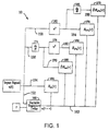
- FIG. 1 is a block diagram of an analog signal processor for detecting and classifying deterministic properties of observed data using correlation parameters, according to the present invention.
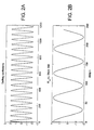
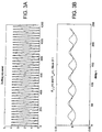
- FIG. 2B is a graph of a correlation parameter versus time delay ⁇ , generated by an auto-correlator (block 164 ) of FIG. 1, based on the input signal of FIG. 2 A.
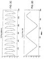
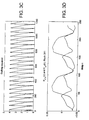
- FIG. 2D is a graph of a correlation parameter versus time delay ⁇ , generated by an auto-correlator (block 164 ) of FIG. 1, based on the input signal of FIG. 2 C.
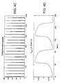
- FIG. 3A is a graph of an output signal representing the square of the input signal of FIG. 2A generated by a squaring device (block 182 ) of FIG. 1 .
- FIG. 3B is a graph of a correlation parameter generated by a correlator (block 170 ) of FIG. 1, based on the input signal of FIG. 2 A and the squared signal of FIG. 3 A.
- FIG. 3C is a graph of an output signal representing the square of the input signal of FIG. 2C generated by a squaring device (block 182 ) of FIG. 1 .
- FIG. 3D is a graph of a correlation parameter generated by a correlator (block 170 ) of FIG. 1, based on the input signal of FIG. 2 C and the squared signal of FIG. 3 C.
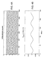
- FIG. 4A is a graph of an output signal representing the square of the derivative of input signal of FIG. 2A generated by a derivative device (block 174 ) and a squaring device (block 178 ) of FIG. 1 .
- FIG. 4B is a graph of a correlation parameter generated by a correlator (block 168 ) of FIG. 1, based on the input signal of FIG. 2 A and the squared derivative signal of FIG. 4 A.
- FIG. 4C is a graph of an output signal representing the square of the derivative of input signal of FIG. 2C generated by a derivative device (block 168 ) and a squaring device (block 178 ) of FIG. 1 .
- FIG. 4D is a graph of a correlation parameter generated by a correlator (block 168 ) of FIG. 1, based on the input signal of FIG. 2 A and the squared derivative signal of FIG. 4 C.
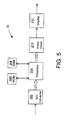
- FIG. 5 is a block diagram of a digital signal processor for detecting and classifying deterministic properties of observed data using correlation parameters that are based on nonlinear dynamical principles, according to the present invention.
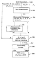
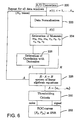
- FIG. 6 is a flow chart showing a process for implementing, using the digital processor of FIG. 5, a simple digital detector for detecting determinism and/or nonlinearity, according to the present invention.
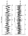
- FIG. 7A is a graph of an deterministic signal generated by a Rössler model in 0 dB Gaussian noise.
- FIG. 7B is a graph a signal segment of pure Gaussian noise.
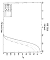
- FIG. 8A is a graph of probability of detection for a linear model coefficient a 2 versus noise level in decibels for three levels of probability of false alarm.
- FIG. 8B is a graph of probability of detection for a nonlinear model coefficient a 3 versus noise level in decibels for three levels of probability of false alarm.
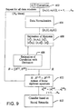
- FIG. 9 is a flow chart showing a process for implementing an acoustic signal classifier for multi-class target recognition, using the digital processor of FIG. 5, according to the present invention.
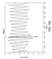
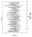
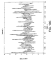
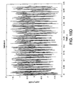
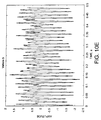
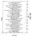
- FIGS. 10A-F are graphs of acoustic amplitude, versus time, of six differing mobile land vehicles, respectively, approaching a closet point of approach from left at a speed of 15 miles per hour.
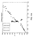
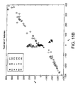
- FIGS. 11A-B are graphs of a 1 parameter values versus a 2 parameters values for training and test data sets, respectively, for the six differing mobile land vehicles of FIGS. 10A-F, according to the present invention.
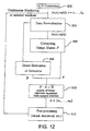
- FIG. 12 is a flow chart showing a process for implementing an acoustic signal classifier for detailed characterization of transient (non-stationary) underwater signals, using the digital processor of FIG. 5, according to the invention.
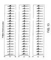
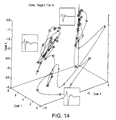
- FIG. 13 is a graph of echo-location pulses, versus time, generated by a dolphin.
- FIG. 14 is a three dimensional graph showing the values of three of the five available estimated model coefficients for the pulses shown in FIG. 13 .
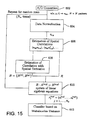
- FIG. 15 is a flow chart showing a process for implementing a spatial pattern or image recognition system based on dynamical generator models, using the digital processor of FIG. 5, according to the invention.
- FIG. 16A is a plot of a random field of image data.
- FIG. 16B is a plot of image data generated by numerically solving a set of wave equations.
- FIG. 16C is the image data of FIG. 16B corrupted by 100% noise shown in the plot of FIG. 16 A.
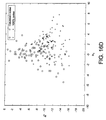
- FIG. 16D is a graph of a, parameter values verses a 2 parameters values for the corrupted image of FIG. 16A, indicated by the symbol ( ⁇ ), and the random image data of FIG. 16C, indicated by the symbol (+).
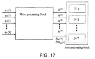
- FIG. 17 is a flow diagram of general signal processing techniques showing correlations for coefficient estimation and showing post-processing according to the present invention.
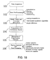
- FIG. 18 is a block diagram showing the general signal processing scheme, according to the invention, for revealing deterministic properties of observed data signals.
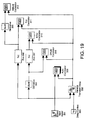
- FIG. 19 is a schematic of a general analog signal processor for detecting and classifying deterministic properties of observed data signals using correlation parameters.
- the present invention is embodied in a signal processing apparatus, and related method, for detecting and classifying aspects of dynamical information or observed data signals that reflect deterministic properties of the data signals using an efficient estimation technique for determining correlation parameters based on nonlinear dynamical principles.
- the signal processing apparatus implements a technique that is capable of detecting and classifying very general structure in the observed data.
- the technique is particularly advantageous for detecting and classifying observed data derived from complicated chaotic or nonlinear time evolution which may be spectrally broadband and very difficult to detect using any standard signal processing and transform methods.
- the estimation technique may be applied to a wide variety of observed data for detailed characterization of transient (non-stationary) air or underwater signals, including acoustic signal classification for multi-class target recognition.
- the correlation parameters may be selected to reveal deterministic properties based on nonlinear dynamical principles, or the correlation parameters may be based on heuristically selected nonlinear dynamical models represented by delayed and/or coupled differential equations.
- the signal processing apparatus of the invention may be embodied in an analog circuit device 10 , shown in FIG. 1, for providing general deterministic signal discrimination of general scalar input signals based on a delay-differential signal model up to a quadratic order.
- the analog circuit device is based on the architecture of Section 2.1 below, with the function transformation f(u) being set to u 2 .
- the analog circuit device 10 estimates observed data feature correlations using a circuit of operational amplifiers and correlators.
- the analog circuit device provides high computational speed and efficiency. Visual inspection of the resulting correlation parameters also provides high speed classification by a human operator, or alternately, simple statistical tests may be used on the resulting correlation parameters to provide simple feature comparisons.
- An example input signal u(t) is provided to the analog circuit device using autonomous Van Der Pol circuit oscillations.
- the analog circuit device 10 receives the input signal u(t) and provides it to a plurality of signal processing paths 152 , 154 , 156 and 158 .
- a first path 152 the input signal is delayed by a predetermined time period ⁇ (tau) by a variable transport delay 160 to generate a delayed input signal u(t ⁇ ).
- the variable transport delay may be implemented using a Digitally Programmable Delay Generator (Part No.: AD9500) available from Analog Devices, Inc. of Norwood, Mass.
- the delayed input signal u(t ⁇ ) is provided by a signal path 162 to a series of correlators 164 , 166 , 168 , 170 and 172 for correlation with the input signal or with processed forms of the input signal.
- the correlators each may be implemented using a CMOS Digital Output Correlator (Part No.: TMC2023) available from Fairchild Semiconductor, Inc. of South Portland, Me.
- the first correlator 164 is provided with the input signal u(t) from the second signal processing path 154 and with the delayed input signal u(t ⁇ t) and generates a first correlation parameter signal based on a correlation of the input signals.
- the first correlation parameter signal is an autocorrelation of the input signal u(t) and is designated R uu (t) and corresponds to the correlation parameter of Eqn. 27 below.
- a third signal path 156 is coupled to a derivative device 174 that generates from the input signal u(t) a derivative signal du/dt on a signal path 176 .
- the derivative device is implemented using an operational amplifier (not shown) configured with resistor and capacitor elements as known in the art.
- the second correlator 116 receives the derivative signal du/dt and the delayed input signal u(t- ⁇ ) and generates a second correlation parameter signal which is designated D ⁇ circumflex over ( ) ⁇ Ruu(t) and which corresponds to the correlation parameter of Eqn. 28 below.
- the derivative signal du/dt is also provided to a squaring device 128 which generates a squared derivative signal (du/dt) 2 on a signal path 180 .
- the third correlator 168 receives the squared derivative signal (du/dt) 2 and the delayed input signal u(t ⁇ ) and generates a third correlation parameter signal which is designated Ru u(dot)u 2 u ( ⁇ ) and which corresponds to the correlation parameter of Eqn. 30 below.
- the fourth signal path 158 is coupled to a squaring device 182 which generates a squared signal u 2 on a signal line 184 .
- the fourth correlator 170 receives the squared signal from the squaring device and receives the delayed input signal u(t ⁇ ) and generates a fourth correlation parameter signal which is designated DR u 2 u ( ⁇ ) and which corresponds to the correlation parameter of Eqn. 32 below.
- the squared signal is also provided to a derivative device 186 which generates a derivative squared signal on a signal line 188 .
- the fifth correlator 172 receives the derivative squared signal d(u 2 )/dt and the delayed input signal u(t ⁇ ) and generates a fifth correlation parameter signal which is designated D ⁇ circumflex over ( ) ⁇ R u 2 u ( ⁇ ) and which corresponds to the correlation parameter of Eqn. 34 below.
- the parameter ⁇ represents the nonlinear dissipation in the input signal.
- the input signal evolves as a simple harmonic oscillator (FIG. 2 A).
- FIGS. 2-4 The response of the analog circuit device 10 is demonstrated by the graphs shown in FIGS. 2-4.
- Shown in FIG. 3A is the square of the simple harmonic signal of FIG. 2A, versus time delay ⁇ , generated by the squaring device (block 182 ).
- Shown in FIG. 4A is the derivative squared of the simple harmonic signal of FIG. 2A, versus time delay ⁇ , generated by the derivative device (block 186 ).
- FIG. 2 C Shown in FIG.
- 3C is the squared nonlinear signal of FIG. 2C, versus time delay ⁇ , generated by the squaring device (block 132 ).
- Shown in FIG. 4C is the derivative squared nonlinear signal of FIG. 2A, versus time delay ⁇ , generated by the derivative device (block 186 ).
- the values of the correlations (FIGS. 2B, 3 B and 4 B) are very harmonic or sinusoidal and the values of the nonlinear correlations (FIGS. 3B and 4B) tend to be small
- the nonlinear regime FIGS. 2C, 3 C and 4 C
- the values of the correlations (FIGS. 2D, 3 D and 4 D) have peculiar shapes and the nonlinear correlations are significantly larger.
- FIGS. 5-8 Another embodiment of the invention based on a digital signal processing technique for revealing deterministic properties of observed data signals is shown with respect to FIGS. 5-8.
- the technique is implemented using a digital signal processor 20 (FIG. 5) that includes an analog-to-digital converter 202 , a processor 204 , read only memory (ROM) 206 , random access memory (RAM) 208 , a video driver 210 , and a display 212 .
- the digital signal processor may be implemented using a general purpose processor such as, for example, an IBM compatible personal computer using processing software such as Matlab supra. Alternately, the digital signal processor may be a special purpose processor, a gate array or a programmable digital processing unit such as the ADSP-210xx family of development tools provided by Analog Devices, Inc.
- An analog signal is digitized by the A/D converter 202 generating a series of data values of length L w (block 220 , FIG. 6 ).
- the data values are normalized (block 222 ) and used to calculated an estimation of moments (block 224 ).
- the normalization technique is discussed in more detail in Section 2.2 below.
- the estimates are derived from a dynamical model based on the delayed differential equation of Eqn. 9 below.
- the moment estimations forms a correlation matrix R of A Eqn. 23 below.
- An estimation of correlations with derivatives is used to estimate a derivative B matrix (block 226 ) of Eqn. 21 below.
- the individual derivative correlations are estimated using Eqns. 49-51 below.
- the model coefficient parameters are provided to a threshold process (block 230 ).
- the threshold process uses existing discrimination techniques such as statistics and averaging to distinguish the deterministic signals from random noise (block 232 ).
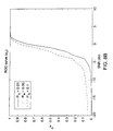
- ROC receiver operating characteristics
- threshold values for coefficients a 2 and a 3 used to generate ROC curves of FIGS. 8A and 8B are shown in Table 1 (below) for 0 dB noise and different pairs of probability of detection P d and probability of false alarm P fa .
- FIG. 9 Another embodiment of the invention is shown in FIG. 9, which is similarly based on a digital processing technique, detects deterministic properties of two observed data signals from two sensors.
- This digital signal processing technique has been shown to be particularly advantageous for vehicle acoustic signature detection.
- the technique is similarly implemented using the digital signal processor 20 (FIG. 5 ).
- the two observed signals, x 1 (i) and x 2 (i) are digitized (block 402 ) and the digital data signals are normalized (block 404 ).
- An estimation of moments is performed (block 406 ), based on the delayed differential equations shown in Appendix A Eqns. 60 and 61, generating an R matrix shown in Appendix A Eqn. 62.
- the A matrix 72 and 73 is calculated (block 408 ) and used with the R matrix to calculate (block 410 ) the A matrix in accordance with Appendix A, Eqns. 81 and 82.
- the A matrix is repeated for all data windows N w .
- the A matrix is provided to a classifier which is implemented through a neural network (block 412 ).
- the post-processing decision scheme is provided by a Learning Vector Quantization (LVQ) neural net classifier.
- the LVQ may be constructed using the NeuralNet toolbox of the Matlab software.
- functions of the neural net toolbox which may be used include: initlvq, trainlvq, and simulvq.
- the standard Matlab syntax is used.
- the feature vector output from the above processing chain corresponding to N targets are written as 5 ⁇ N w input matrices A 1 , A 2 , . . . AN.
- the Matlab processing algorithm then consists of the following:
- the input vector is formed:
- the index of targets is formed:
- each index 1, 2, . . . N is repeated Nw times.
- the index is then transformed into vectors of targets:
- S 2 is the number of known target classes.
- the size of the competitive neural net hidden layer S 1 is chosen. Typically, this is at least several times the number of targets.
- W 1 is a S 1 ⁇ 5 weight matrix for competitive layer and W 2 is a S 2 ⁇ S 1 weight matrix for the linear layer which are obtained during initializing:
- the network is then trained:
- a single 5-dimensional input vector of features A is chosen corresponding to some observed signal, and input to the network, which then makes a decision quantified as the output of the linear output layer:
- FIGS. 10A-10F Sample acoustic recordings from 6 mobile land vehicles, shown in FIGS. 10A-10F, respectively, were used to test the classification of the 6 vehicles. All land vehicles are moving left to right at a speed of 15 km/hr. The sampling frequency is 1024 Hz.
- Table 2 (below) which comprises a “confusion matrix”, indicating the correct and incorrect classification decisions output by the neural net, based on the true input classes. The table shows that the neural net classifier provides the correct class decision in most cases.
- FIG. 12 Another embodiment of the invention based on a digital signal processing technique for revealing deterministic properties of observed data signals is shown in FIG. 12 .
- This embodiment is based on the architecture of Section 2.4 of Appendix A and is particularly advantageous for analyzing non-stationary dolphin echo-location signals.
- the analog location signals are digitized (block 502 ) by the A/D converter 202 (FIG. 5) and resulting digitized signals are normalized (block 504 ).
- a design matrix F is composed (block 506 ) based on the model specification given in Appendix A Eqn. 9.
- the derivative matrix B is estimated directly from the normalized data (block 508 ).
- the correlation coefficient matrix A is calculated (block 510 ).
- the correlation coefficient is used by post-processing steps (block 512 ) such as those discussed with respect to Appendix A, FIG. A- 2 , block 106 . This process may be applied to monitoring a continuous data stream or applied to selected data windows.
- the test data consists of a pulse train of short transient acoustic pulses, shown in FIG. 13, produced by dolphins as they attempt to echo-locate objects in an ocean environment.
- the results, in the form of a feature trajectory, are shown on an operator's display and are illustrated by FIG. 14. A systematic search strategy during the first few dolphin pulses is evident.
- FIG. 15 Another embodiment of the invention based on a digital signal processing technique for revealing deterministic properties of observed data signals is shown in FIG. 15 .
- This embodiment is based on the architecture of Section 2.5 of Appendix A and is particularly advantageous for analyzing spatial patterns.
- the image data signals are digitized (block 602 ) by the A/D converter 202 (FIG. 5) and resulting digitized signals are normalized (block 604 ). Rows of data extracted from the image matrix are used as input.
- a spatial correlation matrix R is composed (block 606 ) based on the model specification given in Appendix A Eqns. 86 and 87.
- a spatial derivative matrix B is estimated directly from the normalized data (block 608 ).
- the correlation coefficient matrix A is calculated (block 610 ).
- the correlation coefficient is used by a post processing step (block 612 ) such as a classifier based on a Mahalanobis Distance.
- test data is constructed using the following Matlab commands:
- uxy tri2grid(p,t,u,x,y)
- uxyi interp 2 (x, y, uxy, xi, yi, ‘cubic’)
- FIG. 16 B A graphical plot showing the 2D image produced by these commands is shown in FIG. 16 B.
- the random field is generated with the following Matlab commands:
- the algorithmic device is intended to sense local structure in the continuous field constituting the image. Hence, to avoid possible biases due to boundary conditions and spurious symmetries in the data, we construct a set of data (observation) window constructed by choosing a random set of rows (or columns) of the image.
- the model coefficients of Appendix A Eqn. 86 are estimated using the correlation method described in Section 1.1.
- the independent variable is the x-index of the image. Otherwise, the algorithmic operations are identical to the procedure of Section 1.1 in which the independent variable is time.
- the input data consists of a 513 ⁇ 513 pixel image, and 100 observation windows are chosen using random rows to generate a data ensemble.
- the algorithm outputs an ensemble of 5 dimensional feature vectors corresponding to Block 105 of FIG. A- 2 .
- Two such distributions of feature vectors are obtained, corresponding, respectively, to the purely random and noisy wave equation data.
- the (a 1 , a 2 ) projection of these two ensembles is plotted in FIG. 16 D. In this case, the local dynamical structure of the noisy wave equation is sensed, and is apparent by the separation of the two feature distributions.
- a finite dimensional dynamical model can be described by a system of:
- ⁇ denotes an integro-differential operator
- the input of the system is a data stream (temporal, spatial, or spatio-temporal) x ⁇ x 1 ,x 2 , . . . ⁇ , which can be either scalar or multivariate.
- the set of model parameters ⁇ A ⁇ is usually estimated using an optimization technique, which minimizes a cost function, which can be defined as:
- ⁇ for example, can be an L 2 norm.
- the technique is called a least-squares minimization.
- DDEs Delayed Differential Equations
- Eq. (1) is a subclass of Eq. (5) when all delays are zero.
- the much wider solution family of DDEs allows us to describe a great variety of signals, which cannot be represented by finite-dimensional ODEs.
- the processing method is not restricted to any particular signal class or generator.
- j 1, . . . , V ⁇ used to estimate coefficients. All these outputs can be post-processed using F- 1 , F- 2 , . . . , F- 7 techniques described in the text. The following are examples of implementations for each corresponding component in the processing scheme:
- A-1 continuously measured data x(t), or data digitized while recording from single or multiple sensors, including acoustic, optical, electromagnetic, or seismic sensors, but not restricted to this set; the process of digitizing transforms an independent continuous variable into its discrete version: t ⁇ t i t 0 +(i ⁇ 1) ⁇ t, where ⁇ t is the sampling interval, which defines a time scale for the incoming data;
- A-2 data retrieved from a storage device such as optical or magnetic disks, tapes and other types of permanent or reusable memories
- a stream of analog data, or a set of digitized scalar or vector data is obtained and this data set may contain information to be detected, classified, recognized, modeled, or to be used as a learning set.
- This becomes a set of ordered numbers in case of scalar input x(i) ⁇ x(i), where the index i 1, 2 . . . , L can indicate time, position in space, or any other independent variable along which data evolution occurs.
- x(i) we will also refer to x(i) as an “observation” or “measurement” window.
- the signal in continuous form (where necessary) we will denote the signal as a continuous (analog) function x(t) of independent variable t, t ⁇ [T 1 T 2 ].
- ⁇ k (j) (X) ⁇ is a set of scalar basis functions for the j-th component of F.
- ⁇ dot over (x) ⁇ F[x,x ⁇ ]+a 1 x+a 2 x ⁇ +a 3 x 2 +a 4 xx ⁇ +a 5 x ⁇ 2 (9)
- i 1, . . . , L ⁇ as input.
- Coefficients can be estimated in a data window by forming a cost function and minimizing the model error, Eq. (4), using e.g. a least-squares technique. Alternately, we may use a coefficient estimation scheme based on computing correlation functions.
- estimating the dynamical model requires explicit or implicit estimation of the signal derivative. This may be performed directly in the analog domain. Alternately, here are several algorithms which can be optionally used to estimate continuous derivatives in a digital domain d/dt ⁇ circumflex over (D) ⁇ :
- (2d+1) is the number of points taken for the estimation, ⁇ t is the time (or length, if the derivative is spatial) between samples;
- D-2 higher-order estimators for example, cubic algorithms
- quadratic for example, a sum of absolute values of differences between the derivative and its estimate
- this estimator is sensitive to even small amounts of noise; such sensitivity can be useful for detecting weak noise in a smooth background of low-dimensional deterministic signals.
- D-4 discrete-time dynamical models e.g. nonlinear regression models
- x ( i +1) F A ( x ( i ), x ( i ⁇ ), . . . , x ( i ⁇ m )) (18)
- R ⁇ ( ⁇ x 2 ⁇ R xx ⁇ ( ⁇ ) ⁇ x 3 ⁇ R x 2 ⁇ x ⁇ ( ⁇ ) R xx 2 ⁇ ( ⁇ ) R xx ⁇ ( ⁇ ) ⁇ x 2 ⁇ R x 2 ⁇ x ⁇ ( ⁇ ) R xx 2 ⁇ ( ⁇ ) ⁇ x 3 ⁇ ⁇ x 3 ⁇ R x 2 ⁇ x ⁇ ( ⁇ ) ⁇ x 4 ⁇ R x 3 ⁇ x ⁇ ( ⁇ ) R x 2 ⁇ x 2 ⁇ ( ⁇ ) R x 2 ⁇ x ⁇ ( ⁇ ) R xx 2 ⁇ ( ⁇ ) R x 3 ⁇ x ⁇ ( ⁇ ) R x 3 ⁇ x ⁇ ( ⁇ ) R x 2 ⁇ x ⁇ ( ⁇ ) R xx 2 ⁇ ( ⁇ ) R x 3 ⁇ x
- Our classification features being the estimated coefficients in the model expansion, may be constructed using the equations connecting the dynamical correlations with the correlation matrix. Together they form a generalized set of correlations.
- M 1,2,3,4,5 (such as in the model Eq.
- the solution can be expressed analytically by calculating determinants of R and using Cramer's rule.
- the analytic solution is typically not practical and robust numerical methods must be used (see Press, W. H., et al. “Numerical recipes in C: the art of scientific computing” Cambridge University Press, Cambridge, New York, 1988, for LU-decomposition, SVD and other relevant techniques).
- the correlation matrix R( ⁇ ) and the vector of dynamical correlations B( ⁇ ) can also be output as a result of the data processing described above. Its classification capability can be enhanced by letting r change over some range ⁇ min to ⁇ max and using the entire function.
- the total output of the core processing block for one data window consists of the feature vectors ⁇ A( ⁇ )
- ⁇ [ ⁇ min , ⁇ max ] ⁇ and correlation matrices ⁇ R( ⁇ )
- ⁇ [ ⁇ min , ⁇ max ] ⁇ calculated for different values of the delay ⁇ .
- a typical useful range of delays is [1, L eff /10].
- a series of data windows is mapped into feature and correlation distributions, which are subject to post-processing described in the next block.
- classifiers such as that known in the art based on Mahalanobis distances (for example, Ray, S., and Turner, L. F. Information Sciences 60, p.217).
- F-4 by building threshold detectors in feature space based on standard signal processing schemes, for example, the Neyman-Pearson criterion (Abed-Meraim, K., Qiu, W., Hua, Y. “Blind System Identification”, Proceedings of the IEEE 85(8), p. 1310, 1997; McDonough, R., and Whalen, A. “Detection of Signals in Noise”, Academic Press, 1995);
- Histograms are the most widely used density estimator. The discontinuity of histograms can cause extreme difficulty if derivatives of the estimates are required. Therefore, in most applications a better estimator (such as kernel density estimators) should be chosen.
- Goal Provide discrimination of general scalar input signals based on continuous dynamical models.
- Analog Circuit processor with scalar analog inputs.
- Model Class Based on Delay-Differential Signal Model up to quadratic order.
- Post-Processing Visual inspection of correlation functions, and (optional) statistical t -test for hypothesis testing.
- Analog circuit consisting of operational amplifiers and correlators.
- Design Details The design is outlined in FIG. 19 .
- the functions of the various components are:
- Block 301 Analog Data Input Port.
- the data input stream is denoted by u. It is convenient to normalize data to zero mean and unit variance. Such normalization allows us to avoid large amplitude variations in the processing chain and to make correlations comply with conventional definitions.
- Block 302 Transport Delay Generator with adjustable delay time ⁇ , providing a delayed datastream u(t ⁇ ).
- Block 303 Delay Control. Provides a set-up circuit for the Transport Delay Generator. It can be manually controlled by an operator, or automatically tuned using feedback from Blocks 308 - 312 (the link is not shown).
- Block 304 - 305 Analog Derivative. These two identical blocks take the signal as input and output its time derivative as a transform. Though the function of this block is similar to what is computed in Eq. (?), there are many other possible implementation of this block including known analog circuits based on operational amplifiers.
- An important variable parameter for this Block is a derivative smoothing range, which is analogous to the parameter d in Eq. (5). It should provide a variable smoothing range for the signal derivative. Without smoothing (weighted integration) the derivative may greatly amplify noise characteristics, which may degrade quality of the computation and visualization in Blocks 308 - 312 (Correlators).
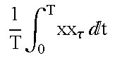
- T is the window length or “accumulation time”.
- the Blocks 308 - 312 output R u 1 u 2 for visualization, and/or (optionally) for further post-processing.
- correlators may span a range of delays set by Block 303 , such as [ ⁇ , ⁇ max ]. In this case, their output will be a function R u 1 u 2 ([ ⁇ , ⁇ max ]) rather than a single number per window T.
- the correlation functions can be transformed into a video signal and shown on a monitor for an operator's inspection.
- T, d, ⁇ , ⁇ max parameters in the processing chain (T, d, ⁇ , ⁇ max ), which may require tuning by an operator, or by automatic adjustment using a feedback optimization routine discussed below.
- Block 310 Correlation of Functionally Transformed Signal Derivative.
- Block 311 Correlation of Functionally Transformed Signal.
- Block 312 Derivative of Correlation of Functionally Transformed Signal.
- the analog device as a whole can be replicated to process several input data streams in parallel. It can also be used to compute “reverse” correlations. For example, R u 2 u has its “reverse” counter-pair R uu 2 . This can be done simply by putting ⁇ 0 (i.e. advanced variables) in Blocks 302 - 303 . Alternately, this can be done by swapping the delayed and direct circuits.
- Simple statistical post-processing can be added to the device to perform two functions:
- N w windows of data we have a set of N w ⁇ M features. They each can be either vectors (for a range of delays ⁇ ) or numbers (single delay).
- I x (y,z) is the incomplete beta function.
- the significance is a number between zero and one, and is the probability that
- Goal Provide detection of possible deterministic structure, and simultaneously nonlinear structure, in a highly noisy digital scalar input signal.
- Model Class Delay-Differential Equation Signal Model up to quadratic order.
- Post-Processing Detection Theoretic threshold detector, specifically a Neyman-Pearson detector, designed using estimated model coefficients (features).
- This design is intended to provide a simple and parsimonious architecture for the detection of unknown deterministic signals (e.g. sinusoids, or broadband nonlinear processes) in highly noisy environments.
- the model class (a quadratic DDE) can be optimized to particular input signal classes.
- the output of the processor is the estimated DDE model coefficients, which are then used as features for a detection theoretic threshold method.
- the Neyman-Pearson threshold detector implemented below provides standard receiver operating characteristic (ROC) curves, summarizing detection performance. Hypothesis testing on input signals is accomplished by simple comparison with the feature threshold.
- Detector Design using known data or data properties, we estimate the feature distributions, calculate appropriate thresholds ⁇ overscore (a) ⁇ k (j) , and assess performance characteristics (ROC-curves).
- PDF Probability Density Function
- Multi-variate threshold detectors can also be built using several features by implementing either a joint probability framework or simply numerically estimating the P d by counting events of correct and false detection by trial-and-error.
- Goal Provide detailed target classification based on linear and nonlinear signal properties, for acoustic signals from various land vehicles.
- Model Class System of Ordinary Differential Equations, two degrees-of-freedom, quadratic order.
- Post-Processing Five dimensional feature space with multi-target feature distributions, and a neural net architecture for target class decision output.
- This design is intended to provide a simple and parsimonious architecture for the detailed classification of acoustic signatures.
- the data is derived from mechanical systems (land vehicles) and has known linear and nonlinear properties.
- the estimated model coefficients are used to construct a five-dimensional feature space, and a neural net architecture is then used on this space to provide post-processing decision making.
- X ⁇ x 1 (i) ⁇ x(i),x 2 (i) ⁇ x(i ⁇ )
- ⁇ dot over (x) ⁇ 1 a 1 (1) x 1 +a 2 (1) x 2 +a 3 (1) x 1 2 +a 4 (1) x 1 x 2 +a 5 (1) x 2 2 (60)
- ⁇ dot over (x) ⁇ 2 a 1 (2) x 1 +a 2 (2) x 2 +a 3 (2) x 1 2 +a 4 (2) x 1 x 2 +a 5 (2) x 2 2 (61)
- Goal Provide detailed waveform classification based on linear and nonlinear signal properties, for transient acoustic echo-location signals from marine mammals.
- Model Class Delay-Differential Equation Signal Model up to quadratic order.
- Post-Processing Five dimensional feature space with simple operator visualization.
- This design is intended to provide a simple and parsimonious architecture for the detailed characterization of transient acoustic signatures.
- the data is derived from a series of echo-location chirps emitted by dolphins during their target discrimination search.
- the estimated model coefficients of the DDE model provide detailed characterization of the waveform of each chirp. Because the chirp's waveforms change in time, the model coefficients (features) show a systematic trajectory in the feature space. Simple operator visualization provides insight into this search procedure.
- This device is designed to process short transient signals (pulses).
- the design is similar to the “Simple Digital Detector for Determinism and/or Nonlinearity” (Section 2.2).
- Samses Pulses
- the design is similar to the “Simple Digital Detector for Determinism and/or Nonlinearity” (Section 2.2).
- Samses Pulses
- the design is similar to the “Simple Digital Detector for Determinism and/or Nonlinearity” (Section 2.2).
- Samps Simple Digital Detector for Determinism and/or Nonlinearity”
- Step 2 instead of composing a correlation matrix, we compose a design matrix F (see, for example, “Numerical Recipes in C” by W. H. Press et.al., Cambridge University Press, 1992, page 671). It has column elements which are algebraically constructed from input data values, and the different rows represent different instances of observation.
- the rule used to compose column elements is defined by the expansion given in the right hand side of Eq. (9).
- the unknown coefficients ⁇ a 1 , . . . , a 5 ⁇ in the expansion are classification features which must be estimated as follows: for the input ⁇ x 1 (i),x 2 (i)
- i 1, . . .
- Goal Provide detailed pattern recognition of 2D digital images based on the dynamical properties of a possible underlying spatio-temporal process.
- Model Class Delay-differential equation in the spatial coordinate.
- This design is intended to provide a simple and parsimonious architecture for the discrimination and classification of 2D digital images.
- the underlying premise is that some component of the spatio-temporal image structure is generated by a continuous physical or man-made process that can be approximately modeled by a delay-differential equation in the spatial coordinates.
- the DDE model can therefore capture information about the spatial dynamical coupling using generalized correlations of the image intensities. This type of processing may be particularly appropriate for images generated by natural phenomena, such as SAR of the sea surface.
- the synthetic input data consists of a solution to the continuous wave equation restricted to a square domain.
- the data may be constructed using the Partial-Differential Equation Toolbox of the Matlab processing environment (“Matlab 5”, scientific modeling and visualization software provided by The MathWorks Inc., Natick, Mass. 01760, USA, phone (508)-647-7001).
- ⁇ ⁇ u ⁇ y ⁇ a 1 ⁇ u ⁇ ( x , y , t ) + a 2 ⁇ u ⁇ ( x , y - ⁇ , t ) + ⁇ a 3 ⁇ ( u ⁇ ( x , y , t ) ) 2 + a 4 ⁇ u ⁇ ( x , y , t ) ⁇ u ⁇ ( x , y - ⁇ , t ) + ⁇ a 5 ⁇ ( u ⁇ ( x , y - ⁇ , t ) ) 2 . ( 89 )
Abstract
Description
| TABLE 1 | ||||
| Pfa = 0.01 | Pfa = 0.05 | Pfa = 0.1 | ||
| a2 (P d ± 1) | a2 = 14.62 | a2 = 15.00 | a2 = 15.19 | ||
| a3 | a3 = 0.50 | a3 = 0.70 | a3 = 0.80 | ||
| (Pd = 0.75) | (Pd = 0.84) | (Pd = 0.87) | |||
| TABLE 2 | |||||||
| Vehicle | | Vehicle | Vehicle | ||||
| 1 | |
3 | |
5 | 6 | ||
| |
26 | 0 | 0 | 0 | 0 | 0 |
| |
0 | 23 | 1 | 2 | 0 | 0 |
| |
0 | 3 | 19 | 4 | 0 | 0 |
| |
0 | 1 | 5 | 20 | 0 | 0 |
| |
0 | 0 | 0 | 0 | 26 | 0 |
| |
0 | 1 | 0 | 0 | 0 | 25 |
| TABLE 3 | |||
| a1 | a2 | ||
| 100% moise Mean | 1.73 +/− 0.23 | −11.42 +/− 0.26 | ||
| σ | 2.25 | 2.64 | ||
| pure noise Mean | 0.08 +/− 0.19 | −8.34 +/− 0.47 | ||
| σ | 1.86 | 4.72 | ||
| TABLE 4 | |||||
| |
100% | 200% | 300% | ||
| confidence level | 0.999 | 0.938 | 0.811 | ||


| No. | Definition | Notation | | Digital Alorithm | |
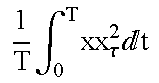
| 1 |
 |
Rxx(τ) | r1 |
 |
|
| 2 |
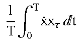 |
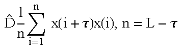
R{dot over (x)}x(τ) | d1 |
 |
|
| 3 |
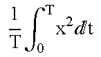 |
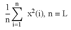
<x2> | m2 |
 |
|
| 4 |
 |
<x3> | m3 |
 |
|
| 5 |
 |
<x4> | m4 |
 |
|
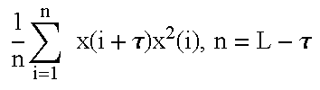
| 6 |
 |
Rx 2 x(τ) | r2 |
 |
|
| 7 |
 |
R xx 2 (τ) | r3 |
 |
|
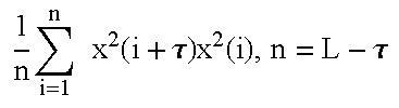
| 8 |
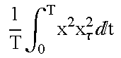 |
Rx 2 x 2 (τ) | r4 |
 |
|
| 9 |
 |
<{dot over (x)}xxτ> | d2 | d2 = 0.5 {circumflex over (D)} |
|
| 10 |
 |
Rxx 2 | d3 |
 |
|
| 11 |
 |
Rx 3 x(τ) | r5 |
 |
|
| 12 |
 |
Rxx 3 (τ) | r6 |
 |
|


Claims (3)
Priority Applications (1)
| Application Number | Priority Date | Filing Date | Title |
|---|---|---|---|
| US10/145,569 US6732064B1 (en) | 1997-07-02 | 2002-05-13 | Detection and classification system for analyzing deterministic properties of data using correlation parameters |
Applications Claiming Priority (4)
| Application Number | Priority Date | Filing Date | Title |
|---|---|---|---|
| US5157997P | 1997-07-02 | 1997-07-02 | |
| US09/105,529 US6278961B1 (en) | 1997-07-02 | 1998-06-26 | Signal and pattern detection or classification by estimation of continuous dynamical models |
| US09/191,988 US6401057B1 (en) | 1997-07-02 | 1998-11-13 | Detection and classification system for analyzing deterministic properties of data using correlation parameters |
| US10/145,569 US6732064B1 (en) | 1997-07-02 | 2002-05-13 | Detection and classification system for analyzing deterministic properties of data using correlation parameters |
Related Parent Applications (1)
| Application Number | Title | Priority Date | Filing Date |
|---|---|---|---|
| US09/191,988 Division US6401057B1 (en) | 1997-07-02 | 1998-11-13 | Detection and classification system for analyzing deterministic properties of data using correlation parameters |
Publications (1)
| Publication Number | Publication Date |
|---|---|
| US6732064B1 true US6732064B1 (en) | 2004-05-04 |
Family
ID=32180360
Family Applications (1)
| Application Number | Title | Priority Date | Filing Date |
|---|---|---|---|
| US10/145,569 Expired - Lifetime US6732064B1 (en) | 1997-07-02 | 2002-05-13 | Detection and classification system for analyzing deterministic properties of data using correlation parameters |
Country Status (1)
| Country | Link |
|---|---|
| US (1) | US6732064B1 (en) |
Cited By (49)
| Publication number | Priority date | Publication date | Assignee | Title |
|---|---|---|---|---|
| US20040117043A1 (en) * | 2002-09-07 | 2004-06-17 | Igor Touzov | Optimized calibration data based methods for parallel digital feedback, and digital automation controls |
| US20050180638A1 (en) * | 1997-12-29 | 2005-08-18 | Glickman Jeff B. | Energy minimization for classification, pattern recognition, sensor fusion, data compression, network reconstruction and signal processing |
| US20060084881A1 (en) * | 2004-10-20 | 2006-04-20 | Lev Korzinov | Monitoring physiological activity using partial state space reconstruction |
| US20070044072A1 (en) * | 2005-08-16 | 2007-02-22 | Hayles Timothy J | Automatically Generating a Graphical Data Flow Program Based on a Circuit Diagram |
| US20070219453A1 (en) * | 2006-03-14 | 2007-09-20 | Michael Kremliovsky | Automated analysis of a cardiac signal based on dynamical characteristics of the cardiac signal |
| US20080015829A1 (en) * | 2006-07-14 | 2008-01-17 | University Of Washington | Statistical analysis of coupled circuit-electromagnetic systems |
| US20080027689A1 (en) * | 2006-07-14 | 2008-01-31 | University Of Washington | Combined fast multipole-qr compression technique for solving electrically small to large structures for broadband applications |
| US20090085873A1 (en) * | 2006-02-01 | 2009-04-02 | Innovative Specialists, Llc | Sensory enhancement systems and methods in personal electronic devices |
| US20090099778A1 (en) * | 2007-10-12 | 2009-04-16 | Gerard Kavanagh | Seismic data processing workflow decision tree |
| US20100204599A1 (en) * | 2009-02-10 | 2010-08-12 | Cardionet, Inc. | Locating fiducial points in a physiological signal |
| US7835889B1 (en) * | 2005-09-06 | 2010-11-16 | The Mathworks, Inc. | Variable transport delay modelling mechanism |
| US20100298656A1 (en) * | 2009-05-20 | 2010-11-25 | Triage Wireless, Inc. | Alarm system that processes both motion and vital signs using specific heuristic rules and thresholds |
| US20110066010A1 (en) * | 2009-09-15 | 2011-03-17 | Jim Moon | Body-worn vital sign monitor |
| US20120158360A1 (en) * | 2010-12-17 | 2012-06-21 | Cammert Michael | Systems and/or methods for event stream deviation detection |
| US8321004B2 (en) | 2009-09-15 | 2012-11-27 | Sotera Wireless, Inc. | Body-worn vital sign monitor |
| US8364250B2 (en) | 2009-09-15 | 2013-01-29 | Sotera Wireless, Inc. | Body-worn vital sign monitor |
| US8437824B2 (en) | 2009-06-17 | 2013-05-07 | Sotera Wireless, Inc. | Body-worn pulse oximeter |
| US8475370B2 (en) | 2009-05-20 | 2013-07-02 | Sotera Wireless, Inc. | Method for measuring patient motion, activity level, and posture along with PTT-based blood pressure |
| US8527038B2 (en) | 2009-09-15 | 2013-09-03 | Sotera Wireless, Inc. | Body-worn vital sign monitor |
| US8545417B2 (en) | 2009-09-14 | 2013-10-01 | Sotera Wireless, Inc. | Body-worn monitor for measuring respiration rate |
| US8591411B2 (en) | 2010-03-10 | 2013-11-26 | Sotera Wireless, Inc. | Body-worn vital sign monitor |
| US8602997B2 (en) | 2007-06-12 | 2013-12-10 | Sotera Wireless, Inc. | Body-worn system for measuring continuous non-invasive blood pressure (cNIBP) |
| US8700366B1 (en) | 2005-09-06 | 2014-04-15 | The Mathworks, Inc. | Variable transport delay modelling mechanism |
| US8740802B2 (en) | 2007-06-12 | 2014-06-03 | Sotera Wireless, Inc. | Body-worn system for measuring continuous non-invasive blood pressure (cNIBP) |
| US8747330B2 (en) | 2010-04-19 | 2014-06-10 | Sotera Wireless, Inc. | Body-worn monitor for measuring respiratory rate |
| US8888700B2 (en) | 2010-04-19 | 2014-11-18 | Sotera Wireless, Inc. | Body-worn monitor for measuring respiratory rate |
| US20140354988A1 (en) * | 2013-05-31 | 2014-12-04 | Canon Kabushiki Kaisha | Method and device for processing data |
| US8979765B2 (en) | 2010-04-19 | 2015-03-17 | Sotera Wireless, Inc. | Body-worn monitor for measuring respiratory rate |
| US9173594B2 (en) | 2010-04-19 | 2015-11-03 | Sotera Wireless, Inc. | Body-worn monitor for measuring respiratory rate |
| US9173593B2 (en) | 2010-04-19 | 2015-11-03 | Sotera Wireless, Inc. | Body-worn monitor for measuring respiratory rate |
| US9339209B2 (en) | 2010-04-19 | 2016-05-17 | Sotera Wireless, Inc. | Body-worn monitor for measuring respiratory rate |
| US9364158B2 (en) | 2010-12-28 | 2016-06-14 | Sotera Wirless, Inc. | Body-worn system for continuous, noninvasive measurement of cardiac output, stroke volume, cardiac power, and blood pressure |
| US9372664B2 (en) | 2012-04-20 | 2016-06-21 | International Business Machines Corporation | Comparing event data sets |
| US9439574B2 (en) | 2011-02-18 | 2016-09-13 | Sotera Wireless, Inc. | Modular wrist-worn processor for patient monitoring |
| CN106017879A (en) * | 2016-05-18 | 2016-10-12 | 河北工业大学 | Universal circuit breaker mechanical fault diagnosis method based on feature fusion of vibration and sound signals |
| US9792259B2 (en) | 2015-12-17 | 2017-10-17 | Software Ag | Systems and/or methods for interactive exploration of dependencies in streaming data |
| US20180156905A1 (en) * | 2016-12-07 | 2018-06-07 | Raytheon Bbn Technologies Corp. | Detection and signal isolation of individual vehicle signatures |
| WO2018120283A1 (en) * | 2016-12-29 | 2018-07-05 | 合肥工业大学 | Simulation circuit fault diagnosis method based on continuous wavelet analysis and elm network |
| US10229092B2 (en) | 2017-08-14 | 2019-03-12 | City University Of Hong Kong | Systems and methods for robust low-rank matrix approximation |
| US20190102718A1 (en) * | 2017-09-29 | 2019-04-04 | Oracle International Corporation | Techniques for automated signal and anomaly detection |
| US10357187B2 (en) | 2011-02-18 | 2019-07-23 | Sotera Wireless, Inc. | Optical sensor for measuring physiological properties |
| US10806351B2 (en) | 2009-09-15 | 2020-10-20 | Sotera Wireless, Inc. | Body-worn vital sign monitor |
| WO2021019776A1 (en) * | 2019-08-01 | 2021-02-04 | Tokyo Institute Of Technology | "Brain-computer interface system suitable for synchronizing one or more nonlinear dynamical systems with the brain activity of a person" |
| US20210365611A1 (en) * | 2018-09-27 | 2021-11-25 | Oracle International Corporation | Path prescriber model simulation for nodes in a time-series network |
| US20210365643A1 (en) * | 2018-09-27 | 2021-11-25 | Oracle International Corporation | Natural language outputs for path prescriber model simulation for nodes in a time-series network |
| US11253169B2 (en) | 2009-09-14 | 2022-02-22 | Sotera Wireless, Inc. | Body-worn monitor for measuring respiration rate |
| US11330988B2 (en) | 2007-06-12 | 2022-05-17 | Sotera Wireless, Inc. | Body-worn system for measuring continuous non-invasive blood pressure (cNIBP) |
| US11607152B2 (en) | 2007-06-12 | 2023-03-21 | Sotera Wireless, Inc. | Optical sensors for use in vital sign monitoring |
| US11896350B2 (en) | 2009-05-20 | 2024-02-13 | Sotera Wireless, Inc. | Cable system for generating signals for detecting motion and measuring vital signs |
Citations (12)
| Publication number | Priority date | Publication date | Assignee | Title |
|---|---|---|---|---|
| US3845288A (en) * | 1971-06-28 | 1974-10-29 | Trw Inc | Data normalizing method and system |
| US3924235A (en) * | 1972-07-31 | 1975-12-02 | Westinghouse Electric Corp | Digital antenna positioning system and method |
| US4912765A (en) * | 1988-09-28 | 1990-03-27 | Communications Satellite Corporation | Voice band data rate detector |
| US5057992A (en) * | 1989-04-12 | 1991-10-15 | Dentonaut Labs Ltd. | Method and apparatus for controlling or processing operations of varying characteristics |
| US5277053A (en) * | 1990-04-25 | 1994-01-11 | Litton Systems, Inc. | Square law controller for an electrostatic force balanced accelerometer |
| US5619432A (en) * | 1995-04-05 | 1997-04-08 | The United States Of America As Represented By The Secretary Of The Navy | Discriminate reduction data processor |
| JPH1032494A (en) * | 1996-07-15 | 1998-02-03 | Sony Corp | Digital signal processing method and processor, digital signal recording method and recorder, recording medium and digital signal transmission method and transmitter |
| US5727128A (en) * | 1996-05-08 | 1998-03-10 | Fisher-Rosemount Systems, Inc. | System and method for automatically determining a set of variables for use in creating a process model |
| US5867807A (en) * | 1995-10-26 | 1999-02-02 | Agency Of Industrial Science & Technology, Ministry Of International Trade & Industry | Method and apparatus for determination of optical properties of light scattering material |
| US6035223A (en) * | 1997-11-19 | 2000-03-07 | Nellcor Puritan Bennett Inc. | Method and apparatus for determining the state of an oximetry sensor |
| US6124134A (en) * | 1993-06-25 | 2000-09-26 | Stark; Edward W. | Glucose related measurement method and apparatus |
| US6564176B2 (en) * | 1997-07-02 | 2003-05-13 | Nonlinear Solutions, Inc. | Signal and pattern detection or classification by estimation of continuous dynamical models |
-
2002
- 2002-05-13 US US10/145,569 patent/US6732064B1/en not_active Expired - Lifetime
Patent Citations (12)
| Publication number | Priority date | Publication date | Assignee | Title |
|---|---|---|---|---|
| US3845288A (en) * | 1971-06-28 | 1974-10-29 | Trw Inc | Data normalizing method and system |
| US3924235A (en) * | 1972-07-31 | 1975-12-02 | Westinghouse Electric Corp | Digital antenna positioning system and method |
| US4912765A (en) * | 1988-09-28 | 1990-03-27 | Communications Satellite Corporation | Voice band data rate detector |
| US5057992A (en) * | 1989-04-12 | 1991-10-15 | Dentonaut Labs Ltd. | Method and apparatus for controlling or processing operations of varying characteristics |
| US5277053A (en) * | 1990-04-25 | 1994-01-11 | Litton Systems, Inc. | Square law controller for an electrostatic force balanced accelerometer |
| US6124134A (en) * | 1993-06-25 | 2000-09-26 | Stark; Edward W. | Glucose related measurement method and apparatus |
| US5619432A (en) * | 1995-04-05 | 1997-04-08 | The United States Of America As Represented By The Secretary Of The Navy | Discriminate reduction data processor |
| US5867807A (en) * | 1995-10-26 | 1999-02-02 | Agency Of Industrial Science & Technology, Ministry Of International Trade & Industry | Method and apparatus for determination of optical properties of light scattering material |
| US5727128A (en) * | 1996-05-08 | 1998-03-10 | Fisher-Rosemount Systems, Inc. | System and method for automatically determining a set of variables for use in creating a process model |
| JPH1032494A (en) * | 1996-07-15 | 1998-02-03 | Sony Corp | Digital signal processing method and processor, digital signal recording method and recorder, recording medium and digital signal transmission method and transmitter |
| US6564176B2 (en) * | 1997-07-02 | 2003-05-13 | Nonlinear Solutions, Inc. | Signal and pattern detection or classification by estimation of continuous dynamical models |
| US6035223A (en) * | 1997-11-19 | 2000-03-07 | Nellcor Puritan Bennett Inc. | Method and apparatus for determining the state of an oximetry sensor |
Non-Patent Citations (1)
| Title |
|---|
| 1992 IEEE Conference on Acoustics, Speech and Signal Processing Mar. 1992 vol. 5, pp. 321-324 "Nonlinear Signal Processing Using Empirical Gl-bal Dynamical Equations", Jeffrey S. Brush et al. * |
Cited By (111)
| Publication number | Priority date | Publication date | Assignee | Title |
|---|---|---|---|---|
| US7272262B2 (en) * | 1997-12-29 | 2007-09-18 | Glickman Jeff B | Energy minimization for classification, pattern recognition, sensor fusion, data compression, network reconstruction and signal processing |
| US20050180638A1 (en) * | 1997-12-29 | 2005-08-18 | Glickman Jeff B. | Energy minimization for classification, pattern recognition, sensor fusion, data compression, network reconstruction and signal processing |
| US20050185848A1 (en) * | 1997-12-29 | 2005-08-25 | Glickman Jeff B. | Energy minimization for classification, pattern recognition, sensor fusion, data compression, network reconstruction and signal processing |
| US7912290B2 (en) | 1997-12-29 | 2011-03-22 | Glickman Jeff B | Energy minimization for classification, pattern recognition, sensor fusion, data compression, network reconstruction and signal processing |
| US7174048B2 (en) * | 1997-12-29 | 2007-02-06 | Glickman Jeff B | Energy minimization for classification, pattern recognition, sensor fusion, data compression, network reconstruction and signal processing |
| US20040117043A1 (en) * | 2002-09-07 | 2004-06-17 | Igor Touzov | Optimized calibration data based methods for parallel digital feedback, and digital automation controls |
| US20060084881A1 (en) * | 2004-10-20 | 2006-04-20 | Lev Korzinov | Monitoring physiological activity using partial state space reconstruction |
| US7996075B2 (en) | 2004-10-20 | 2011-08-09 | Cardionet, Inc. | Monitoring physiological activity using partial state space reconstruction |
| US20070044072A1 (en) * | 2005-08-16 | 2007-02-22 | Hayles Timothy J | Automatically Generating a Graphical Data Flow Program Based on a Circuit Diagram |
| US8782596B2 (en) | 2005-08-16 | 2014-07-15 | National Instruments Corporation | Automatically generating a graphical data flow program based on a circuit diagram |
| US7835889B1 (en) * | 2005-09-06 | 2010-11-16 | The Mathworks, Inc. | Variable transport delay modelling mechanism |
| US8180608B1 (en) * | 2005-09-06 | 2012-05-15 | The Mathworks, Inc. | Variable transport delay modeling mechanism |
| US8700366B1 (en) | 2005-09-06 | 2014-04-15 | The Mathworks, Inc. | Variable transport delay modelling mechanism |
| US8390445B2 (en) | 2006-02-01 | 2013-03-05 | Innovation Specialists, Llc | Sensory enhancement systems and methods in personal electronic devices |
| US7872574B2 (en) | 2006-02-01 | 2011-01-18 | Innovation Specialists, Llc | Sensory enhancement systems and methods in personal electronic devices |
| US20090085873A1 (en) * | 2006-02-01 | 2009-04-02 | Innovative Specialists, Llc | Sensory enhancement systems and methods in personal electronic devices |
| US20110121965A1 (en) * | 2006-02-01 | 2011-05-26 | Innovation Specialists, Llc | Sensory Enhancement Systems and Methods in Personal Electronic Devices |
| US7729753B2 (en) | 2006-03-14 | 2010-06-01 | Cardionet, Inc. | Automated analysis of a cardiac signal based on dynamical characteristics of the cardiac signal |
| US20070219453A1 (en) * | 2006-03-14 | 2007-09-20 | Michael Kremliovsky | Automated analysis of a cardiac signal based on dynamical characteristics of the cardiac signal |
| US20080015829A1 (en) * | 2006-07-14 | 2008-01-17 | University Of Washington | Statistical analysis of coupled circuit-electromagnetic systems |
| US7676351B2 (en) * | 2006-07-14 | 2010-03-09 | University Of Washington | Statistical analysis of coupled circuit-electromagnetic systems |
| US20080027689A1 (en) * | 2006-07-14 | 2008-01-31 | University Of Washington | Combined fast multipole-qr compression technique for solving electrically small to large structures for broadband applications |
| US7933944B2 (en) * | 2006-07-14 | 2011-04-26 | University Of Washington | Combined fast multipole-QR compression technique for solving electrically small to large structures for broadband applications |
| US11330988B2 (en) | 2007-06-12 | 2022-05-17 | Sotera Wireless, Inc. | Body-worn system for measuring continuous non-invasive blood pressure (cNIBP) |
| US11607152B2 (en) | 2007-06-12 | 2023-03-21 | Sotera Wireless, Inc. | Optical sensors for use in vital sign monitoring |
| US9215986B2 (en) | 2007-06-12 | 2015-12-22 | Sotera Wireless, Inc. | Body-worn system for measuring continuous non-invasive blood pressure (cNIBP) |
| US9161700B2 (en) | 2007-06-12 | 2015-10-20 | Sotera Wireless, Inc. | Body-worn system for measuring continuous non-invasive blood pressure (cNIBP) |
| US9668656B2 (en) | 2007-06-12 | 2017-06-06 | Sotera Wireless, Inc. | Body-worn system for measuring continuous non-invasive blood pressure (cNIBP) |
| US8808188B2 (en) | 2007-06-12 | 2014-08-19 | Sotera Wireless, Inc. | Body-worn system for measuring continuous non-invasive blood pressure (cNIBP) |
| US10765326B2 (en) | 2007-06-12 | 2020-09-08 | Sotera Wirless, Inc. | Body-worn system for measuring continuous non-invasive blood pressure (cNIBP) |
| US8740802B2 (en) | 2007-06-12 | 2014-06-03 | Sotera Wireless, Inc. | Body-worn system for measuring continuous non-invasive blood pressure (cNIBP) |
| US8602997B2 (en) | 2007-06-12 | 2013-12-10 | Sotera Wireless, Inc. | Body-worn system for measuring continuous non-invasive blood pressure (cNIBP) |
| US20090099778A1 (en) * | 2007-10-12 | 2009-04-16 | Gerard Kavanagh | Seismic data processing workflow decision tree |
| US20100204599A1 (en) * | 2009-02-10 | 2010-08-12 | Cardionet, Inc. | Locating fiducial points in a physiological signal |
| US8200319B2 (en) | 2009-02-10 | 2012-06-12 | Cardionet, Inc. | Locating fiducial points in a physiological signal |
| US8956293B2 (en) | 2009-05-20 | 2015-02-17 | Sotera Wireless, Inc. | Graphical ‘mapping system’ for continuously monitoring a patient's vital signs, motion, and location |
| US10973414B2 (en) | 2009-05-20 | 2021-04-13 | Sotera Wireless, Inc. | Vital sign monitoring system featuring 3 accelerometers |
| US11918321B2 (en) | 2009-05-20 | 2024-03-05 | Sotera Wireless, Inc. | Alarm system that processes both motion and vital signs using specific heuristic rules and thresholds |
| US8594776B2 (en) | 2009-05-20 | 2013-11-26 | Sotera Wireless, Inc. | Alarm system that processes both motion and vital signs using specific heuristic rules and thresholds |
| US10555676B2 (en) | 2009-05-20 | 2020-02-11 | Sotera Wireless, Inc. | Method for generating alarms/alerts based on a patient's posture and vital signs |
| US8180440B2 (en) | 2009-05-20 | 2012-05-15 | Sotera Wireless, Inc. | Alarm system that processes both motion and vital signs using specific heuristic rules and thresholds |
| US8672854B2 (en) | 2009-05-20 | 2014-03-18 | Sotera Wireless, Inc. | System for calibrating a PTT-based blood pressure measurement using arm height |
| US11896350B2 (en) | 2009-05-20 | 2024-02-13 | Sotera Wireless, Inc. | Cable system for generating signals for detecting motion and measuring vital signs |
| WO2010135518A1 (en) * | 2009-05-20 | 2010-11-25 | Sotera Wireless, Inc. | System that monitors patient motion and vital signs |
| US8738118B2 (en) | 2009-05-20 | 2014-05-27 | Sotera Wireless, Inc. | Cable system for generating signals for detecting motion and measuring vital signs |
| US9492092B2 (en) | 2009-05-20 | 2016-11-15 | Sotera Wireless, Inc. | Method for continuously monitoring a patient using a body-worn device and associated system for alarms/alerts |
| US8475370B2 (en) | 2009-05-20 | 2013-07-02 | Sotera Wireless, Inc. | Method for measuring patient motion, activity level, and posture along with PTT-based blood pressure |
| US20100298656A1 (en) * | 2009-05-20 | 2010-11-25 | Triage Wireless, Inc. | Alarm system that processes both motion and vital signs using specific heuristic rules and thresholds |
| US10987004B2 (en) | 2009-05-20 | 2021-04-27 | Sotera Wireless, Inc. | Alarm system that processes both motion and vital signs using specific heuristic rules and thresholds |
| US11589754B2 (en) | 2009-05-20 | 2023-02-28 | Sotera Wireless, Inc. | Blood pressure-monitoring system with alarm/alert system that accounts for patient motion |
| US20100298660A1 (en) * | 2009-05-20 | 2010-11-25 | Triage Wireless, Inc. | Body-worn device and associated system for alarms/alerts based on vital signs and motion; also describes specific monitors that include barcode scanner and different user interfaces for nurse, patient, etc. |
| US8956294B2 (en) | 2009-05-20 | 2015-02-17 | Sotera Wireless, Inc. | Body-worn system for continuously monitoring a patients BP, HR, SpO2, RR, temperature, and motion; also describes specific monitors for apnea, ASY, VTAC, VFIB, and ‘bed sore’ index |
| US8909330B2 (en) * | 2009-05-20 | 2014-12-09 | Sotera Wireless, Inc. | Body-worn device and associated system for alarms/alerts based on vital signs and motion |
| US10085657B2 (en) | 2009-06-17 | 2018-10-02 | Sotera Wireless, Inc. | Body-worn pulse oximeter |
| US11134857B2 (en) | 2009-06-17 | 2021-10-05 | Sotera Wireless, Inc. | Body-worn pulse oximeter |
| US11103148B2 (en) | 2009-06-17 | 2021-08-31 | Sotera Wireless, Inc. | Body-worn pulse oximeter |
| US8437824B2 (en) | 2009-06-17 | 2013-05-07 | Sotera Wireless, Inc. | Body-worn pulse oximeter |
| US9596999B2 (en) | 2009-06-17 | 2017-03-21 | Sotera Wireless, Inc. | Body-worn pulse oximeter |
| US11638533B2 (en) | 2009-06-17 | 2023-05-02 | Sotera Wireless, Inc. | Body-worn pulse oximeter |
| US8554297B2 (en) | 2009-06-17 | 2013-10-08 | Sotera Wireless, Inc. | Body-worn pulse oximeter |
| US9775529B2 (en) | 2009-06-17 | 2017-10-03 | Sotera Wireless, Inc. | Body-worn pulse oximeter |
| US8622922B2 (en) | 2009-09-14 | 2014-01-07 | Sotera Wireless, Inc. | Body-worn monitor for measuring respiration rate |
| US10123722B2 (en) | 2009-09-14 | 2018-11-13 | Sotera Wireless, Inc. | Body-worn monitor for measuring respiration rate |
| US8545417B2 (en) | 2009-09-14 | 2013-10-01 | Sotera Wireless, Inc. | Body-worn monitor for measuring respiration rate |
| US10595746B2 (en) | 2009-09-14 | 2020-03-24 | Sotera Wireless, Inc. | Body-worn monitor for measuring respiration rate |
| US11253169B2 (en) | 2009-09-14 | 2022-02-22 | Sotera Wireless, Inc. | Body-worn monitor for measuring respiration rate |
| US8740807B2 (en) | 2009-09-14 | 2014-06-03 | Sotera Wireless, Inc. | Body-worn monitor for measuring respiration rate |
| US20110066010A1 (en) * | 2009-09-15 | 2011-03-17 | Jim Moon | Body-worn vital sign monitor |
| US10420476B2 (en) | 2009-09-15 | 2019-09-24 | Sotera Wireless, Inc. | Body-worn vital sign monitor |
| US10806351B2 (en) | 2009-09-15 | 2020-10-20 | Sotera Wireless, Inc. | Body-worn vital sign monitor |
| US8321004B2 (en) | 2009-09-15 | 2012-11-27 | Sotera Wireless, Inc. | Body-worn vital sign monitor |
| US8364250B2 (en) | 2009-09-15 | 2013-01-29 | Sotera Wireless, Inc. | Body-worn vital sign monitor |
| US8527038B2 (en) | 2009-09-15 | 2013-09-03 | Sotera Wireless, Inc. | Body-worn vital sign monitor |
| US8591411B2 (en) | 2010-03-10 | 2013-11-26 | Sotera Wireless, Inc. | Body-worn vital sign monitor |
| US10278645B2 (en) | 2010-03-10 | 2019-05-07 | Sotera Wireless, Inc. | Body-worn vital sign monitor |
| US8727977B2 (en) | 2010-03-10 | 2014-05-20 | Sotera Wireless, Inc. | Body-worn vital sign monitor |
| US10213159B2 (en) | 2010-03-10 | 2019-02-26 | Sotera Wireless, Inc. | Body-worn vital sign monitor |
| US8888700B2 (en) | 2010-04-19 | 2014-11-18 | Sotera Wireless, Inc. | Body-worn monitor for measuring respiratory rate |
| US9173594B2 (en) | 2010-04-19 | 2015-11-03 | Sotera Wireless, Inc. | Body-worn monitor for measuring respiratory rate |
| US9173593B2 (en) | 2010-04-19 | 2015-11-03 | Sotera Wireless, Inc. | Body-worn monitor for measuring respiratory rate |
| US8747330B2 (en) | 2010-04-19 | 2014-06-10 | Sotera Wireless, Inc. | Body-worn monitor for measuring respiratory rate |
| US9339209B2 (en) | 2010-04-19 | 2016-05-17 | Sotera Wireless, Inc. | Body-worn monitor for measuring respiratory rate |
| US8979765B2 (en) | 2010-04-19 | 2015-03-17 | Sotera Wireless, Inc. | Body-worn monitor for measuring respiratory rate |
| US9659063B2 (en) * | 2010-12-17 | 2017-05-23 | Software Ag | Systems and/or methods for event stream deviation detection |
| US20120158360A1 (en) * | 2010-12-17 | 2012-06-21 | Cammert Michael | Systems and/or methods for event stream deviation detection |
| US10722131B2 (en) | 2010-12-28 | 2020-07-28 | Sotera Wireless, Inc. | Body-worn system for continuous, noninvasive measurement of cardiac output, stroke volume, cardiac power, and blood pressure |
| US9380952B2 (en) | 2010-12-28 | 2016-07-05 | Sotera Wireless, Inc. | Body-worn system for continuous, noninvasive measurement of cardiac output, stroke volume, cardiac power, and blood pressure |
| US10722130B2 (en) | 2010-12-28 | 2020-07-28 | Sotera Wireless, Inc. | Body-worn system for continuous, noninvasive measurement of cardiac output, stroke volume, cardiac power, and blood pressure |
| US10722132B2 (en) | 2010-12-28 | 2020-07-28 | Sotera Wireless, Inc. | Body-worn system for continuous, noninvasive measurement of cardiac output, stroke volume, cardiac power, and blood pressure |
| US9364158B2 (en) | 2010-12-28 | 2016-06-14 | Sotera Wirless, Inc. | Body-worn system for continuous, noninvasive measurement of cardiac output, stroke volume, cardiac power, and blood pressure |
| US9585577B2 (en) | 2010-12-28 | 2017-03-07 | Sotera Wireless, Inc. | Body-worn system for continuous, noninvasive measurement of cardiac output, stroke volume, cardiac power, and blood pressure |
| US10856752B2 (en) | 2010-12-28 | 2020-12-08 | Sotera Wireless, Inc. | Body-worn system for continuous, noninvasive measurement of cardiac output, stroke volume, cardiac power, and blood pressure |
| US10357187B2 (en) | 2011-02-18 | 2019-07-23 | Sotera Wireless, Inc. | Optical sensor for measuring physiological properties |
| US9439574B2 (en) | 2011-02-18 | 2016-09-13 | Sotera Wireless, Inc. | Modular wrist-worn processor for patient monitoring |
| US11179105B2 (en) | 2011-02-18 | 2021-11-23 | Sotera Wireless, Inc. | Modular wrist-worn processor for patient monitoring |
| US9372664B2 (en) | 2012-04-20 | 2016-06-21 | International Business Machines Corporation | Comparing event data sets |
| US9377995B2 (en) | 2012-04-20 | 2016-06-28 | International Business Machines Corporation | Comparing event data sets |
| US9310307B2 (en) * | 2013-05-31 | 2016-04-12 | Canon Kabushiki Kaisha | Method and device for processing data |
| US20140354988A1 (en) * | 2013-05-31 | 2014-12-04 | Canon Kabushiki Kaisha | Method and device for processing data |
| US9792259B2 (en) | 2015-12-17 | 2017-10-17 | Software Ag | Systems and/or methods for interactive exploration of dependencies in streaming data |
| CN106017879B (en) * | 2016-05-18 | 2018-07-03 | 河北工业大学 | Omnipotent breaker mechanical failure diagnostic method based on acoustic signal Fusion Features |
| CN106017879A (en) * | 2016-05-18 | 2016-10-12 | 河北工业大学 | Universal circuit breaker mechanical fault diagnosis method based on feature fusion of vibration and sound signals |
| US10353060B2 (en) * | 2016-12-07 | 2019-07-16 | Raytheon Bbn Technologies Corp. | Detection and signal isolation of individual vehicle signatures |
| US20180156905A1 (en) * | 2016-12-07 | 2018-06-07 | Raytheon Bbn Technologies Corp. | Detection and signal isolation of individual vehicle signatures |
| US11280826B2 (en) | 2016-12-29 | 2022-03-22 | Hefei University Of Technology | Analog-circuit fault diagnosis method based on continuous wavelet analysis and ELM neural network |
| WO2018120283A1 (en) * | 2016-12-29 | 2018-07-05 | 合肥工业大学 | Simulation circuit fault diagnosis method based on continuous wavelet analysis and elm network |
| US10229092B2 (en) | 2017-08-14 | 2019-03-12 | City University Of Hong Kong | Systems and methods for robust low-rank matrix approximation |
| US20190102718A1 (en) * | 2017-09-29 | 2019-04-04 | Oracle International Corporation | Techniques for automated signal and anomaly detection |
| US20210365643A1 (en) * | 2018-09-27 | 2021-11-25 | Oracle International Corporation | Natural language outputs for path prescriber model simulation for nodes in a time-series network |
| US20210365611A1 (en) * | 2018-09-27 | 2021-11-25 | Oracle International Corporation | Path prescriber model simulation for nodes in a time-series network |
| WO2021019776A1 (en) * | 2019-08-01 | 2021-02-04 | Tokyo Institute Of Technology | "Brain-computer interface system suitable for synchronizing one or more nonlinear dynamical systems with the brain activity of a person" |
Similar Documents
| Publication | Publication Date | Title |
|---|---|---|
| US6732064B1 (en) | Detection and classification system for analyzing deterministic properties of data using correlation parameters | |
| US6564176B2 (en) | Signal and pattern detection or classification by estimation of continuous dynamical models | |
| Pope et al. | Blind signal separation I. linear, instantaneous combinations: I. linear, instantaneous combinations | |
| Besson et al. | Adaptive detection of a signal known only to lie on a line in a known subspace, when primary and secondary data are partially homogeneous | |
| Chakrabarti et al. | Robust radar target classifier using artificial neural networks | |
| US6401057B1 (en) | Detection and classification system for analyzing deterministic properties of data using correlation parameters | |
| Rekavandi et al. | Robust subspace detectors based on α-divergence with application to detection in imaging | |
| Broder | Quickest detection procedures and transient signal detection | |
| US5511008A (en) | Process and apparatus for extracting a useful signal having a finite spatial extension at all times and which is variable with time | |
| Wen et al. | Modeling of correlated complex sea clutter using unsupervised phase retrieval | |
| Chen et al. | $\textsf {S}^ 3T $: An Efficient Score-Statistic for Spatio-Temporal Surveillance | |
| US6718316B1 (en) | Neural network noise anomaly recognition system and method | |
| Bagwe et al. | Automated Radar Signal Analysis Based on Deep Learning | |
| Lei | Robust detection of radiation threat | |
| Ma et al. | Tracking of maneuvering star-convex extended target using modified adaptive extended Kalman Filter | |
| Muccino et al. | Generalized inversion of the Korteweg–de Vries equation | |
| Blacknell et al. | A comparison of simulation techniques for correlated gamma and K-distributed images for SAR applications | |
| Baker et al. | Likelihood ratio methods for underwater acoustics signal detection | |
| Voskoboynikova et al. | Numerical modeling of posteriori algorithms for the geophysical monitoring | |
| Rosenthal et al. | Model selection via misspecified cramér-rao bound minimization | |
| Leung et al. | A spatial temporal dynamical model for multipath scattering from the sea | |
| Stanek et al. | Performance assessment of frequency plane filters applied to track association and sensor registration | |
| Frakt et al. | A generalized Levinson algorithm for covariance extension with application to multiscale autoregressive modeling | |
| CN116680503B (en) | Satellite signal steady capturing method of double sparse optimized array antenna and related equipment | |
| Coulon et al. | Detection of multiplicative noise in stationary random processes using second-and higher order statistics |
Legal Events
| Date | Code | Title | Description |
|---|---|---|---|
| STCF | Information on status: patent grant |
Free format text: PATENTED CASE |
|
| FEPP | Fee payment procedure |
Free format text: PAYOR NUMBER ASSIGNED (ORIGINAL EVENT CODE: ASPN); ENTITY STATUS OF PATENT OWNER: LARGE ENTITY |
|
| AS | Assignment |
Owner name: KADTKE, JAMES, DISTRICT OF COLUMBIA Free format text: NUNC PRO TUNC ASSIGNMENT;ASSIGNOR:NONLINEAR SOLUTIONS, INC.;REEL/FRAME:018109/0514 Effective date: 20060807 |
|
| AS | Assignment |
Owner name: OMNITURE, INC., UTAH Free format text: ASSIGNMENT OF ASSIGNORS INTEREST;ASSIGNOR:KADTKE, JAMES;REEL/FRAME:018109/0942 Effective date: 20060210 |
|
| FEPP | Fee payment procedure |
Free format text: PAT HOLDER NO LONGER CLAIMS SMALL ENTITY STATUS, ENTITY STATUS SET TO UNDISCOUNTED (ORIGINAL EVENT CODE: STOL); ENTITY STATUS OF PATENT OWNER: LARGE ENTITY |
|
| FPAY | Fee payment |
Year of fee payment: 4 |
|
| AS | Assignment |
Owner name: WELLS FARGO FOOTHILL, LLC, AS AGENT, CALIFORNIA Free format text: SECURITY AGREEMENT;ASSIGNOR:OMNITURE, INC.;REEL/FRAME:022078/0141 Effective date: 20081224 |
|
| AS | Assignment |
Owner name: OMNITURE, INC., UTAH Free format text: RELEASE BY SECURED PARTY;ASSIGNOR:WELLS FARGO FOOTHILL, LLC;REEL/FRAME:023525/0335 Effective date: 20091023 |
|
| AS | Assignment |
Owner name: ADOBE SYSTEMS INCORPORATED, CALIFORNIA Free format text: ASSIGNMENT OF ASSIGNORS INTEREST;ASSIGNOR:OMNITURE, INC.;REEL/FRAME:023538/0077 Effective date: 20091112 Owner name: ADOBE SYSTEMS INCORPORATED,CALIFORNIA Free format text: ASSIGNMENT OF ASSIGNORS INTEREST;ASSIGNOR:OMNITURE, INC.;REEL/FRAME:023538/0077 Effective date: 20091112 |
|
| FPAY | Fee payment |
Year of fee payment: 8 |
|
| FPAY | Fee payment |
Year of fee payment: 12 |