EP0770967A2 - Decision support system for the management of an agile supply chain - Google Patents
Decision support system for the management of an agile supply chain Download PDFInfo
- Publication number
- EP0770967A2 EP0770967A2 EP96202971A EP96202971A EP0770967A2 EP 0770967 A2 EP0770967 A2 EP 0770967A2 EP 96202971 A EP96202971 A EP 96202971A EP 96202971 A EP96202971 A EP 96202971A EP 0770967 A2 EP0770967 A2 EP 0770967A2
- Authority
- EP
- European Patent Office
- Prior art keywords
- inventory
- data
- sales
- frame
- demand
- Prior art date
- Legal status (The legal status is an assumption and is not a legal conclusion. Google has not performed a legal analysis and makes no representation as to the accuracy of the status listed.)
- Withdrawn
Links
Images


Classifications
-
- G—PHYSICS
- G06—COMPUTING; CALCULATING OR COUNTING
- G06Q—INFORMATION AND COMMUNICATION TECHNOLOGY [ICT] SPECIALLY ADAPTED FOR ADMINISTRATIVE, COMMERCIAL, FINANCIAL, MANAGERIAL OR SUPERVISORY PURPOSES; SYSTEMS OR METHODS SPECIALLY ADAPTED FOR ADMINISTRATIVE, COMMERCIAL, FINANCIAL, MANAGERIAL OR SUPERVISORY PURPOSES, NOT OTHERWISE PROVIDED FOR
- G06Q10/00—Administration; Management
- G06Q10/06—Resources, workflows, human or project management; Enterprise or organisation planning; Enterprise or organisation modelling
- G06Q10/063—Operations research, analysis or management
- G06Q10/0631—Resource planning, allocation, distributing or scheduling for enterprises or organisations
- G06Q10/06315—Needs-based resource requirements planning or analysis
-
- G—PHYSICS
- G06—COMPUTING; CALCULATING OR COUNTING
- G06Q—INFORMATION AND COMMUNICATION TECHNOLOGY [ICT] SPECIALLY ADAPTED FOR ADMINISTRATIVE, COMMERCIAL, FINANCIAL, MANAGERIAL OR SUPERVISORY PURPOSES; SYSTEMS OR METHODS SPECIALLY ADAPTED FOR ADMINISTRATIVE, COMMERCIAL, FINANCIAL, MANAGERIAL OR SUPERVISORY PURPOSES, NOT OTHERWISE PROVIDED FOR
- G06Q10/00—Administration; Management
- G06Q10/06—Resources, workflows, human or project management; Enterprise or organisation planning; Enterprise or organisation modelling
- G06Q10/063—Operations research, analysis or management
- G06Q10/0637—Strategic management or analysis, e.g. setting a goal or target of an organisation; Planning actions based on goals; Analysis or evaluation of effectiveness of goals
-
- G—PHYSICS
- G06—COMPUTING; CALCULATING OR COUNTING
- G06Q—INFORMATION AND COMMUNICATION TECHNOLOGY [ICT] SPECIALLY ADAPTED FOR ADMINISTRATIVE, COMMERCIAL, FINANCIAL, MANAGERIAL OR SUPERVISORY PURPOSES; SYSTEMS OR METHODS SPECIALLY ADAPTED FOR ADMINISTRATIVE, COMMERCIAL, FINANCIAL, MANAGERIAL OR SUPERVISORY PURPOSES, NOT OTHERWISE PROVIDED FOR
- G06Q30/00—Commerce
- G06Q30/02—Marketing; Price estimation or determination; Fundraising
- G06Q30/0201—Market modelling; Market analysis; Collecting market data
- G06Q30/0202—Market predictions or forecasting for commercial activities
-
- Y—GENERAL TAGGING OF NEW TECHNOLOGICAL DEVELOPMENTS; GENERAL TAGGING OF CROSS-SECTIONAL TECHNOLOGIES SPANNING OVER SEVERAL SECTIONS OF THE IPC; TECHNICAL SUBJECTS COVERED BY FORMER USPC CROSS-REFERENCE ART COLLECTIONS [XRACs] AND DIGESTS
- Y10—TECHNICAL SUBJECTS COVERED BY FORMER USPC
- Y10S—TECHNICAL SUBJECTS COVERED BY FORMER USPC CROSS-REFERENCE ART COLLECTIONS [XRACs] AND DIGESTS
- Y10S706/00—Data processing: artificial intelligence
- Y10S706/902—Application using ai with detail of the ai system
- Y10S706/925—Business
Definitions
- the present invention is directed to a system for supporting management decisions associated with manufacturing of service supply chains that span from a point of creation to a point of consumption and, more particularly, is directed to a system that allows the various decision makers in the supply chain to view the supply chain from their own perspective, obtain information and evaluate decisions concerning past, current and future performance with respect to a diverse set of often conflicting goals.
- a view a Decision Support Frame
- PSI production, sales and inventory
- a decision support system for the management of agile supply chains that provides an architecture including a server side and a client side.
- the server side includes a decision support system database that interfaces with one or more model engines that perform analytical processes on the data to determine requirements and make projections.
- the server side includes a server manager that coordinates requests for service and information.
- the client side includes Decision Support Frames that present the various view points available in the system to the users. A frame manager that coordinates the requests from Decision Support Frame (view points) is provided by the system to access the needed data and models.
- FIG. 1 DSS System Architecture in the Context of Manufacturing Supply Chains.
- FIG. 1 DSS System Architecture in the Context of Equipment Repair Supply Chains.
- FIG. 4 The Data Spaces in Supply Chain Management.
- FIG. 5 Structural Elements in the DSS Database for the Manufacturing Supply Chain.
- FIG. 6 Structural Elements in the DSS Database for the Equipment Repair Supply Chain.
- Figure 11 Data Space Associations of the Demand Management Frame.
- Figure 12 Process Flow of the Demand Management Frame.
- Figure 13 Process Flow of Order Fulfillment.
- Figure 14 Data Flow for the Demand Management Frame.
- Figure 15 Data Space Associations of the Production-Sales-Inventory Planning Frame.
- Figure 16 Process Flow of the Production-Sales-Inventory Planning Frame.
- Figure 17 Data Flow for the Production-Sales-Inventory Planning Frame.
- Figure 18 Data Space Associations of the Supply Management Frame.
- FIG. 19 Process Flow of the Supply Management Frame.
- Figure 20 Data Flow for the Supply Management Frame.
- Figure 21 Data Flow for the Supply Management Frame.
- FIG. 22 Data Space Associations of the Vendor Managed Replenishment Frame.
- FIG. 23 Process Flow of the Vendor Managed Replenishment Frame.
- FIG. 24 Data Flow for the Vendor Managed Replenishment Frame.
- FIG. 1 Data Space Associations of the Distribution Network Design Frame.
- FIG. 26 Process Flow of the Distribution Network Design Frame.
- Figure 27 Data Flow for the Distribution Network Design Frame.
- FIG. 33 System Level Services, the Seven Modules and Model Engine Utilities.
- Figure 36 High level object representation of the system integrator portion of the frame manager.
- Figure 38 Data Flow Diagram for the Supply Chain Network Configurator.
- Figure 40 Hierarchical Structure of a Scenario.
- Figure 41 Data Flow Diagram for the Performance Simulator.
- FIG. 43 Sample Screen from PSI DSS.
- Figure 49 The Opening Screen of the DSS.
- Figure 51 The Select Data Domain Form.
- Figure 60 The Main PSI Frame Form.
- Figure 61 The Options menu choices on the PSI screen.
- Figure 63 The main capacity checking dialog box - The Options tab.
- FIG. 70 Key Component Selection Dialog Box.
- the Decision Support System (DSS) 10 of the present invention relies on quantitative models and data analysis routines to provide decision support.
- PSI production, sales and inventory
- An architecture to provide such support in accordance with the present invention comprises a library of models and routines that are logically linked, regularly updated and maintained.
- the present invention assembles the models and routines in a flexible manner, as needed by a decision making environment, to enable the DSS 10 to provide customized decision support with a readily upgradable and scalable library.
- the architecture of the Decision Support System (DSS) 10 for a manufacturing supply chain is shown in figure 1 and comprises the principal design elements of: a DSS Database 12 with a Database Management System (DBMS) 14 and Supply Chain Information Systems 15, Decision Support Frames 16 which provides the various supply chain view points, a User Interface 18, a Model Engine 20 including various Model Engine Utilities (processes) 22 and a Supply Chain Frame Manager 24.
- the architecture of the DSS 10 in the context of an equipment repair supply chain is illustrated in figure 2.
- the DSS architecture comprises two basic mode divisions: the Client Mode 30 and the Server Mode 32. These modes can be classified with respect to an implementation of the DSS 10 in a supply chain. From a design standpoint the Client Mode 30 is the portion of the DSS architecture that is specific and therefore customizable to provide decision support for any particular decision process and decision maker.
- the Server Mode 32 is the kernel of the DSS architecture that remains largely the same across different applications of the DSS 10 within a given supply chain. Hence, for a given implementation of the client-server DSS architecture in a supply chain, there will be one Server Mode 32 and a number of Client Modes to provide support for the decision processes.
- the Client Mode 30 comprises the User Interface 18, the Decision Support Frames 16, and the client version of the Supply Chain Frame Manager 24.
- the Server Mode 32 comprises the Supply Chain Frame Manager 24, the system level services, the Model Engine 20, and the DSS Database 12.
- the Supply Chain Frame Manager 24, as a participant in both modes, serves to tie the Client and the Server Modes of the architecture together.
- the client-server architecture makes the overall design both extensible (new functionality can be added by customizing a frame in the Client Mode 30) and scalable (new models and routines can be added to the Model Engine 20 in the Server Mode 32). Additionally this design is networkable; one can visualize the Server Mode 32 of the DSS 10 hosted by a server workstation in a client-server network while a number of Client Modes 30 of DSS 10 are hosted in the client computers.
- the layered design of the architecture in terms of how the principal design elements of the DSS 10 are positioned within the architecture, provides a more resilient and stable backbone for decision support.
- the high level design architecture is independent of any computing and networking platform and hence applicable to a variety of environments.
- the structure maintains the design of the horizontal layers for its key system elements while its functionality is more aligned vertically.
- the overall DSS 10 interfaces with the Supply Chain Information Systems 15 through the data exchanges between these systems and the DSS Database 12.
- the DSS 10 has a User Interface 18 to interact with end users through interactive and visual data exchange.
- the main body of the DSS 10 includes the following horizontal layers: User Interface 18; Decision Support Frames 16; Supply Chain Frame Manager 24 (Client and Server); Model Engine 20; and DSS Database 12 .
- the above layers of the DSS 10 can be partitioned into client and Server Modes.
- the system layers within the Client Mode 30 serve an interpretive role between the system data and analytic processing support and the specific end user's decision support needs.
- Those layers under the Server Mode 32 contain system functionalities common to a diversity of users and decision support problems, and usually require more dedicated, higher performance system processing capabilities.
- the DSS 10 will invoke a vertical decision support thread 40 going through visual objects of a User Interface 18, decision logic and what-if scenario manager in a Decision Support Frame, Supply Chain Frame Managers, models or analysis routines in the Model Engine 20 and appropriate data elements in the DSS Database 12.
- An example of a decision support thread 40 is shown by the bi-directional arrows in figure 3.
- the distinguishing characteristic between the manufacturing and repair environments is the degree to which the environment focuses on the production of new goods versus the repair of old ones.
- the equipment repair supply chain has complex reentrant flows, while the manufacturing is characterized by the linear material flows from material procurement to final consumption.
- the DSS Database 12 is internal to the DSS 10 implementation.
- the main objective of the DSS Database 12 is to support the execution of the decision support functionality of the DSS 10. It contains the synthesized data drawn from a variety of external supply chain information sources and Supply Chain Information Systems 15. It may also maintain a set of data unique to the DSS 10 but not available in any existing Supply Chain Information Systems 15. An example of such unique data is the data derived through the analysis of synthesized data.
- the DSS Database 12 can be interfaced to the Supply Chain Information Systems 15 to retrieve the required data and provide updated data, as needed.
- the Database Management System 14 communicates with the Model Engine 20 to provide the input data, and update the database 12 based on the output of the Model Engine 20.
- the DBMS 14 does not duplicate the transaction-based functionality that is typically featured in the Supply Chain Information Systems 15, unless it is critical for decision support needs.
- a structural data representation of the data in various data spaces 50, 52 and 54 (see figure 4) is used to model the elements of the supply chain that are relatively static. Specifying these data elements typically specifies the infrastructure of the supply chain. At the highest level of abstraction, four principal nodes (see figures 5 and 6) in the supply chain 58 are identified:
- Key components 63 are supplied by component suppliers 64 tied to specific component supply nodes 62.
- Production resources 65 produce the various products 66.
- the production resources can be aggregated into production resource groups 67, and are located at production nodes 61.
- Products 66 are the end items that are produced and, based on their various attributes, can be grouped into various product groups 67. These products are stocked at various stock locations identified with inventory nodes 60 and inventory headers 68.
- Customers 69 can be grouped by various criteria into customer groups 70 and demand various products. Customers 69 are located at the demand nodes 59.
- Markets 71 are defined for a cross-section of customers and products.
- Such a data representation in the form of a network of nodes and the ability to group the various constituent elements, provide the flexibility to specify and reconfigure a variety of supply chains.
- a data space is a fundamental domain to characterize basic data elements associated with the supply chain management: demand, supply and inventory data.
- the data spaces 50, 52 and 54 tie the structural data to the process data. It has three principal dimensions: Product/Component; Time; and Node related structural element.
- the node-related structural element can be a customer, an inventory location, or a production resource.
- the data in each data space can be at any resolution (in terms of level of aggregation) along the three dimensions and can be expressed as a quantity or value.
- each point in the data space characterizes the resolution of the product (or component), the time and the node-related structural element.
- a product when describing the aggregate production plan data, a product can be at the resolution of product, time at a resolution of week, and the node-related structural element (Production resource in this case) at a resolution of production resource group.
- a product in describing bottom-up forecasts, can be at the resolution of product, time at a resolution of month, and node related structural element at the resolution of customer.
- This data space 50 has three dimensions: Customer; Product; and Time.
- Customer can be at a resolution of customer or customer group or demand node.
- Product can be at the resolution of product or product group.
- Time can be at a resolution of day, week, bi-week, month, bi-month, quarter or year.
- This data space 52 has the following three dimensions: Production Resource; Product/Component; and Time.
- Production resource can be at a resolution of production resource, production resource group, or production node.
- Product/Component can be at the resolution of component, product or product group.
- Time can be at a resolution of day, week, bi-week, month, bi-month, quarter or year.
- Inventory Data Space 54 This data space 54 has the following three dimensions associated with it: Inventory Location; Product/Component; and Time. Inventory location can be at a resolution of stock location or inventory node. Product/Component can be at the resolution of component, product or product group. Time can be at a resolution of day, week, bi-week, month, bi-month, quarter or year.
- a decision process relates or transforms data either within a data space or between data spaces. For example, aggregate production planning transforms data from the supply space to inventory space and vice versa. We will employ this data space representation to specify the various decision processes in supply chain management.
- the DSS Database 12 comprises structural information (information related to relatively static information such as product groups, market groups, supply chain network, etc.), and process information (dynamic information related to demand, production plan, etc.).
- Figure 5 previously discussed, graphically represents the structural data tables for the manufacturing supply chain.
- the DSS Database 12 for the equipment repair supply chain (see figure 6) comprises structural information (information related to relatively static information such as equipment, repair resources, supply chain network, etc.), and process information (dynamic information related to usage, requirements, repair plan, etc.).
- structural information information related to relatively static information such as equipment, repair resources, supply chain network, etc.
- process information dynamic information related to usage, requirements, repair plan, etc.
- the structural elements are flexibly collected into different groups to allow users to analyze data at various resolutions. For example, equipment of the same age can be grouped together to analyze the effect of age on repair requirements.
- Figure 6 graphically represents the structural data tables for the equipment repair supply chain.
- the process data in the DSS Database 12 are contained in two closely related table type data structures (see below): (I) header file that specifies the resolutions and values on the relevant dimensions of product, customer, time, resource, and item, (ii) corresponding data file which contains the actual data at the resolutions and values specified in the header.
- the process data are preferably stored in these two tables (Table 2, Table 3), rather than one consolidated table (Table 1), to avoid redundancy and updating anomalies. A loss-less join of the header and the data tables will result in the consolidated table (Table 1). The following example demonstrates this point.
- the data tables in the DSS Database 12 are preferably specified as follows: Name of the table; Brief description of the data contained in the table; Identifier for the data fields; Type of the data field; and Brief description of the data fields (this includes the choice of values for the data in this field, if applicable).
- the specifications of the data tables for the manufacturing and equipment repair supply chains can be found in Appendices A and B, respectively.
- the list of the preferred tables in the DSS Database 12 for these chains is as follows: Aggregate Production Plan Data; Aggregate Production Plan Header; Budget Data; Budget Header; Calendar; Component; Component Accommodation Matrix; Component Requirement Data; Component Requirement Header; Component Supplier; Component Supply Contract; Component Supply Node; CPRD Table; Customer; Customer Group; Customer Group; Definition; Customer Orders; DataField Definition; Demand History Data; Demand History Header; Demand Node; Demand Orientation Data; Demand Orientation Header; Domain; Domain Definition; Feature Choices; Forecast Data; Forecast Header; Freight Rate; Inventory Data; Inventory Header; Inventory Node; Inventory Parameters; Market Data; Market Header; Material Delivery Schedule Data; Material Delivery Schedule Header; Planning BOM; POS Data; POS Header; Product; Product Features; Product Group; Product Group Definition; Production Accommodation Matrix; Production Capa
- the present invention preferably provides core reports that support business decision processes by characterizing the link between the various data elements and processes. They synthesize the data and information used in the decision making processes. Associated with each key business process, we will demonstrate the data flow relationships that are used to construct the various forms and reports.
- Some of the preferred forms and reports relevant to the DSS 10 are: Sales Plan; Customer-Demand History; Production-Sales-Inventory Plan; Master Production Plan; Production Capacity Plan; Replenishment Schedule; Customer-DC Assignment; and Supply-DC Assignment
- a Frame 16 is an integrated decision support environment based on an abstraction of the supply chain designed to address a set of related decision problems within a decision process.
- a Frame 16 is therefore defined based on the vantage point or view point of the users along a supply chain. This implies that a frame exists if and only if there are users with specific needs in the supply chain.
- a Frame 16 is a mechanism that unifies the user dialog and display, the models and analysis routines, and data in a manner that is consistent to support the underlying supply chain abstraction of the user.
- Table 4 A summary of the frame concept from both a user and a system perspective is shown in Table 4.
- a Frame 16/72 is the abstraction of the supply chain from a user's point of view. It essentially contains as its design elements a user dialog 72 and user display 74 and a decision logic 76.
- the user dialog 73 and the display 74 contain the form and style of the User Interface 18.
- the decision logic 76 permits the assembly of models and analysis routines and the associated data to address the set of related decision problems.
- the user dialog 72 and display 74 are customized to the specific needs of the PSI planning process, which further determines the design of the User Interface 18 associated with the PSI Planning Frame 160.
- the decision logic 76 in the PSI frame may assemble models and routines from the Model Engine 20 along with the associated data.
- the decision logic 76 in a frame interacts with the Supply Chain Frame Manager 24 to execute the models and routines.
- the Supply Chain Frame Manager 24 then provides the performance feedback to the user.
- a supply-chain-wide view and the necessary Management 80 is recognized by all levels of the management as being vital to managing the business.
- decision makers at different levels and points along the supply chain are primarily motivated by their individual roles and responsibilities. The broader a decision maker's responsibilities, the more likely the decision maker is interested in employing decision support capabilities that target the entire supply chain. The user requirements discussed below for decision support are posed from a supply-chain-wide perspective.
- assessments in business conditions impact one part of the supply chain assess the potential impact on the other parts of the supply chain. Given different future business scenarios, determine their financial consequences across the supply chain. For the enterprise's supply chain which includes major retailers, determine the appropriate division of responsibilities for all partners in the supply chain. Develop and implement performance incentives that will enhance and encourage supply-chain-wide thinking and decision making in the enterprise.
- Demand Management 81 is the process by which the customers' requirements are characterized with the specification of prevailing uncertainty.
- the process involves the development and maintenance of medium-term customer (bottom-up) forecasts. These forecasts are initially developed in periodic joint meetings or communications between the decision makers of the enterprise and the customers. Subsequently, these forecasts are input into the enterprise's supply management system to obtain product allocation approval (place-keeping order). As the actual purchase orders arrive, the enterprise attempts to fulfill the requirements to their customers' satisfaction. We have identified the user requirements discuss below for decision support for this process. Synthesize information from different sources in order to manage the demand requirements effectively, e.g., accessing point-of-sales (POS) data and comparing these with shipment history and customer forecasts. For key customers, develop customer-specific sales forecasts based on historical shipment and sell-through data. Link POS data, where available, to the historical promotion information to analyze the real impact of promotion activities on demand, as opposed to relying on the estimates provides by the retailers.
- POS point-of-sales
- PSI Planning 82 is a process to determine a set of feasible sales, production and inventory requirements for medium to long-term capacity and resource planning for the logistics operations.
- an initial PSI plan can be developed based on the long-term top-down sales forecast and budget plans.
- the planning process then becomes a continuous effort to update the existing PSI plan to accommodate the changes in the requirements before and after a series of monthly PSI planning meetings whose participants include decision makers representing all key functional areas at the enterprise.
- the meetings integrate the inputs from various sources, resolve possible conflicts, and balance the concerns of different functions in order to reconcile, develop and approve a new set of feasible sales, production and inventory requirements.
- the process represents a focal point for the entire logistics planning process, and interacts and coordinates with all major decision making processes.
- Supply Management 83 is a process to determine the production (supply) plan to meet the production (supply) requirements generated by the PSI Planning process.
- the process involves component procurement and factory production planning based on the PSI plans and their changes.
- the production line capacities are created based on long-term product plans, i.e., planned new product release.
- the process continuously updates the production (supply) plan based on changes in the production (supply) requirements generated in the PSI process.
- VMR Vendor Managed Replenishment
- VMR 84 is a process in which the supplier takes on the responsibility of managing the inventory at the customer site for the products it supplies. This process operates on point-of-sales demand as opposed to demand forecasts provided by the customers. VMR involves formulating the contractual agreements between the enterprise and the retailers as well as determining the operating parameters such as shipment quantities and replenishment frequencies. We have identified the user requirements discussed below for decision support for this process. Develop a strategic analysis tool to determine mutually beneficial VMR contracts based on financial and logistics factors. Develop the replenishment plan based on factors such as sell-through and inventory information provided by the retailer, promotion activities, product availability and transportation cost trade-offs.
- the equipment repair supply chain 90 includes the operating location 92, i.e., the point-of-use, the repair shop 94, and the component suppliers 96.
- the demand (or the "requirements") are generated by equipment failures.
- the failed module is replaced from the stock at the operating location 92, and the failed module is eventually sent to the repair shop 94 for repair.
- a module is made up of repair items which in turn are made up of components.
- the repair is carried out by the repair resources (people and machinery). During the repair process at the repair shop 94, certain repair items and components are replaced. Based on the repair needs, repair items and components will be ordered from the sources of supply by the repair shops.
- Equipment Operating Location 92 At the equipment operating location 92, personnel may replace only certain repair items of the module, instead of the whole module These replacement repair items may come from the stock or from other failed modules. This process encourages consolidation of failed modules at the operating location. In the consolidation process, the broken repair item of a broken module is replaced by a good repair item from another broken module. This process may be motivated by the structure of the repair cost function and the need for quick repair. In some cases, due to the fixed costs of sending individual modules to the repair shop, modules are batched to a certain level, before they are sent to the repair shop for a complex overhaul.
- the repair shop 94 is responsible for all the major repairs.
- the type of repair to perform is driven by the level of good modules at the repair location.
- the stock level may drop below the target level, thus triggering a repair request to bring the stock level up to the target level.
- This target level is determined with the objective of maximizing the equipment availability and minimizing the repair costs.
- Component and capacity requirements corresponding to a repair request should be feasible with respect to component availability and resource capacity levels at the repair shop.
- the equipment repair supply chain has clear parallelism with the manufacturing supply chain where the repair items correspond to products and components correspond to materials.
- Equipment operating locations are similar to retailers and equipment is like customers.
- the repair shop is analogous to a production facility.
- modules are made up of repair items, modules correspond to product groups.
- the repair requirements management process is analogous to demand management, and repair supply management to supply management. Similar to the PSI process, there exists a reconciliation process in the equipment repair supply chain to ensure balance between requirements and supply.
- the equipment located at various operating locations are the aircraft operating at the various bases.
- the modules correspond to the Line Replaceable Units, or LRUs and the repair items correspond to Shop Replaceable Units (SRUs).
- SRUs Shop Replaceable Units
- the function of the base is to provide immediate support to the aircraft located at that base, with the objective of maximizing availability of aircraft.
- bases stock good units of replaceable items, called serviceables, so as to be able to replace a failed LRU of an aircraft immediately.
- a base usually, is not involved in major repairs.
- Managing the repair requirements refers to deciding when and which defective items the base will send to the depot for repair with the objective of maximizing the availability of aircraft located at the base and minimizing total cost of repair (which includes a fixed cost component).
- a depot is responsible for all the major repairs.
- the type of repair to perform is driven by the level of good repairable items at the depot.
- the stock level may drop below the target level, thus triggering a repair request to bring the stock level up to the target level.
- This target level also called the Consolidated Serviceable Inventory (CSI) level, is determined by the depot with the objective of maximizing its service level and minimizing its repair costs. Component and capacity requirements corresponding to a repair request should be feasible with respect to component availability and resource capacity levels at the depot.
- CSI Consolidated Serviceable Inventory
- Table 5 below presents the analogy and nomenclature between the equipment repair supply chain, and the manufacturing supply chain with examples from defense and commercial environments.
- the supply chain comprises (see figure 9) the following three decision processes: Requirements Management Process 98; Requirements-Supply Reconciliation Planning Process 100; and Supply Management Process 102.
- the Requirements Management Process 98 concentrates on the activities associated with requirements estimation.
- the objective of this process is to estimate future repair requirements generated by equipment failures.
- Equipment has several repairable parts and equipment failures are caused by failures of the repairable parts.
- estimating future requirements refers to the process of estimating failures of the equipment and of the repairable parts that caused the failures. This is done to estimate repair time requirements (determined in Requirements-Supply Reconciliation Planning Process) and equipment availability at equipment locations, both of which depend on the part that has failed.
- Requirements can be analyzed in two levels: Lower level requirements, called the Raw Requirements, correspond to all repair requirements of the equipment and upper level requirements, called the Consolidated Requirements, correspond to requirements requested from the repair shop, since equipment locations may prefer accumulating their repair requirements and sending them to the repair shop according to certain rules instead of sending them as they occur, or may prefer carrying out minor repairs within the location, with the aim of reducing the fixed and variable costs of repair.
- Raw requirements would correspond to Point of Sales (POS) data and consolidated requirements to retailer order data from the production facility.
- POS Point of Sales
- the bottom-up estimation approach estimates the raw requirements first and then generates the consolidated requirements from raw requirement estimates.
- relationships are determined between failure rates and activity schedules of the equipment. For example, the time to failure of an equipment can be a function of the number of hours it has operated and its maintenance schedule. Once the relationships between failure rates and activities are established by regression or time series models, future failure rates can be estimated based on the planned activity schedules of the equipment.
- the next step is to go to the upper level and estimate consolidated requirements, that is requirements as seen by the repair shop (assuming that repair shop does not have access to raw requirements data). Consolidated requirements depend on what frequency the operating location will send its repair requests to the repair shop.
- the top-down estimation approach makes use of historical data to estimate consolidated requirements.
- Statistical forecasting techniques can be used to support this process.
- the two estimates obtained by bottom-up and top-down approaches are compared, analyzed and reconciled to generate final estimates for consolidated repair requirements.
- the output of this process is the estimated consolidated requirements for an equipment operating location.
- the second process is the Requirements-Supply Reconciliation Planning process 100 that aims at developing an integrated repair plan for the repair shop through a reconciliation process.
- the type and parameters of the repair policy of the repair shop are to be determined.
- Aggregate repair requirements are generated based on the repair policy of the repair shop and estimated consolidated requirements for all facilities.
- the next step is to generate an aggregate repair plan based on repair time estimates for each repairable part and the aggregate repair requirements.
- Feasibility of the aggregate repair plan is checked with respect to resource constraints which are repair resource capacities and key component availability. If the aggregate repair plan is not feasible with respect to resource constraints, then causes for infeasibility are identified and the infeasibility is removed by either changing the level of the resource constraints or moving aggregate requirements forward or backward in time.
- the supply management 102 (see figure 9) is a process to determine the repair plan considering repair people, test equipment and key components. It starts by the translation of the aggregate repair plan into a detailed plan concerning repair resources (repair persons and test equipment), and component requirements. Based on these requirements and the capacity constraints for the repair resources, repair personnel and key components, a detailed repair plan is developed using an optimized based modeling approach. The detailed repair plan is used to generate the key component delivery schedule to be transmitted to the component suppliers.
- the supply management process 102 is also concerned with the development of appropriate procurement policies for key components in terms of identifying the policies, and deriving the corresponding policy parameters.
- the basic Frames 16 of the present invention collectively provide coverage for the overall supply chain.
- the specific instances of these Frames 16 in a particular DSS 10 implementation depend largely on the constituent supply chain, the underlying business processes, and the organizational structure.
- the Demand Management Frame 130 supports the demand management decision process described here.
- Figure 11 shows the participating modules and the associated data spaces for this frame.
- the Demand Management Frame 130 requires the participation of two modules: the Sales Forecasting and Planning (SFP) Module 132 and the Market Data Analysis (MDA) module 134.
- SFP Sales Forecasting and Planning
- MDA Market Data Analysis
- the SFP Module 132 in the Demand Management Frame 130 essentially operates in the D data space, i.e., it transforms data within the conceptual demand data domain.
- the MDA Module 134 in the Demand Management Frame 130 operates in the I and the D data spaces and relates the I data space to the D data space, i.e., it may transform data within the individual D data space as well as transform data from the I data space to the D data space.
- the data space representation of the Demand Management Frame 130 is the union of the data space representations of each participating module, and the interactions among participating modules.
- figure 11 can be complemented by the process flow diagram for this frame, described next, that will detail the connections between the constituent modules and the associated data tables.
- the process flow diagram for the Demand Management Frame 130 is shown in figure 12.
- the modules, data tables, and the principal activities within the scope of this frame are clearly marked by the grooved double-lined border. Only the data tables that are updated by the frame are considered to be within the scope of the frame 130. Other frames, activities and data tables that are related are also shown for completeness.
- the Order Fulfillment 149, that is out-of-scope of the Demand Management Frame 130 but related to it, is shown separately in figure 13 for purposes of clarity. This representation of interaction between Frames 16 is consistent with the interaction between decision processes shown in figure 8.
- the Demand Management Frame 130 supports the functional requirements described below.
- Demand Characterization - Demand data from various sources such as Demand History Data 136, POS Data 138, Market Data 140, and Promotion Data 142 as well as top-down and bottom-up Forecast Data 146 obtained by buyers and account managers will be consolidated and synthesized by the MDA Module 134 and the SFP Module 132.
- Bottom-up Demand Forecasting - Demand Review 144 consolidates demand information received directly from the customer along with the input from the MDA Module 134 and then develops Demand Orientation Data 148.
- the SFP Module 132 will then use Demand Orientation Data 148 as well as other inputs, e.g. Promotion 142 and POS 138 Data, to develop the customer-centric bottom-up forecasts in Forecast Data 146.
- Top-down Forecasting The SFP Module 132 will use market and industry-wide trend analysis performed by the MDA Module 134 along with the enterprise's shipment history to generate the product-centric top-down forecasts in Forecast Data 146.
- Sales Promotion Analysis The MDA Module 134 reviews the demand history from POS Data 138 and Demand History Data 136 along with the customer promotion information from Promotion Data 142 to analyze the impact of promotions on sales. The results of such an analysis are then used to help adjust sales forecasts to account for promotions.
- Forecast Performance Evaluation Using Demand Orientation Data 146, Demand History Data 136 and Promotion Data 142, the SFP 132 and MDA Module 134 can evaluate the quality of enterprise's forecasts and the customer projections.
- the data flow diagram for the Demand Management Frame 130 is shown in figure 14.
- the Demand Management Frame 130 generates two of the core reports listed earlier, namely, the Sales Plan 152 and the Customer-Demand History 154. For each core report, the associated data tables are shown.
- the dashed line indicates the influence of an out-of-scope (with respect to the Demand Management Frame 130) data table in the development of the report.
- the Customer Orders data table 150 is out-of-scope of the Demand Management Frame 130 but influences the Customer-Demand History report 152.
- Demand Management is the process in which the user determines future requirements based on past requirement history and general information related to the supply chain.
- Demand Management supports the analysis of past demand and of market trends as well as the development of future forecasts.
- Requirement Management is used in place of Demand Management.
- Requirement Management is the process where future requirements are estimated based on an analysis of each equipment's activity and on the projection of past requirement history.
- Demand Management regroups the set of processes by which the user analyzes Market Data 140 and past demand history for the purpose of estimating future demand requirements.
- the outputs of Demand Management include the analysis of past history, future forecasts, the analysis of special activities such as sales promotions, and the analysis of forecast errors.
- Two critical outputs of Demand Management are two different medium term forecasts corresponding to two different views on the dynamics of the processes that generate future requirements: the customer centric forecast - generated at the product level for each customer it incorporates the estimations of future demand provided by each customer (Bottom-up Forecast); and the product centric forecast - generated at the product level, it incorporates the impact of market and industry-wide trends on future demand for each product group (Top-down Forecast).
- the objective of Demand Characterization is to provide the user with an environment where (s)he can access, analyze and synthesize demand data from different sources.
- These data include: Sales History data (that include POS and shipment data), Inventory data (relative to the inventory position of its product at the customer's stocking points), and Market Data 140.
- Market Data 140 correspond to various quantitative information, usually provided by external entities such as Nielsen, that relates to the sales for the type of product considered in the entire market.
- Data Acquisition consists of selecting a Data Domain (specific pairs of customer and product), and choosing the type of data to be displayed (POS, demand history, inventory, Market Data 140). Data can be edited and modified and saved along with results of analysis in a scenario.
- Compute display (tables and graphs), and analyze inventory profile per customer.
- This operation involves the operations discussed below.
- Market Data 140 volume, value, market share
- Create price information list of competitor products per price range.
- the objective of the Bottom-up forecasting is to develop a customer specific sales forecast based on historical shipment to the customer, POS information at the customer location, and the customer's own forecast regarding its future orders.
- Data Acquisition consists of selecting a data Domain (specific pairs of customer and product), and choosing the type of data to be displayed: shipment or POS (when available).
- Forecasts generated in the Bottom-up forecasting frame can be saved back to the DSS Database 12 or alternatively saved as scenario.
- This operation involves the operations discussed below.
- POS or Shipment data Disaggregate yearly forecasts onto each period using seasonality factors at different levels of aggregation: Customer group, Individual customers for all products, and Individual customers for each product.
- the objective of the Top-down forecasting is to develop a product centric sales forecast based on historical demand data and industry analysis that accounts for market-wide trends.
- the data Acquisition consists of selecting a data Domain (specific pairs of customer and product), and choosing the type of data to be displayed: shipment or POS (when available).
- Forecasts generated in the Top-down forecasting frame can be saved back to the DSS Database 12 or alternatively saved as a scenario.
- This operation involves the operations discussed below.
- POS or Shipment data Disaggregate yearly forecasts onto each period using seasonality factors at different levels of aggregation: market level, product group level, and product line level.
- the objective of Sales Promotion Analysis is to analyze the impact of promotional activities. It entails maintaining the promotion calendar, estimating the impact of future promotions and assessing the effect on sales of past promotional activities.
- the promotion calendar is a table in which the various characteristics of past and future promotions are recorded. The knowledge and insights gained in sales promotion analysis are used in adjusting bottom-up and top-down sales forecasts.
- Type of promotion defined by who initiates the promotion: firm, retailer, competitor
- Class of promotion defined by the nature of the promotional activity.
- Partition sales Display actual sales attributable to normal sales, seasonal effect and promotion effect.
- Add promotion in promotion calendar - specify type, class, intensity and time period.
- Forecast Performance Evaluation is to assess the accuracy of past sales forecasts. Forecast accuracy is an important measure for several purposes:
- forecast accuracy of one particular version of the forecast is considered: forecast accuracy of one particular version of the forecast, and average accuracy of n periods ahead forecast.
- the first forecast performance type provides point estimations of forecast accuracy, while the second one is an average estimation of the accuracy as a function of the number of period in advance a forecast is produced.
- Requirements Management is the process of estimating the future requirements of reparable items at the equipment location. This process can be divided into two main sub-processes:
- This approach uses a combination of two models: (1) the first model estimates the raw requirements of an equipment by modeling its failure rate as a function of the equipment's activity (or usage) and (2) the second model estimates the consolidated requirement based on the raw requirements and the consolidation policy.
- This operation involves the operations discussed below.
- Kalman Filter based algorithm for requirements estimation (considered appropriate for forecasting equipment failures).
- Compute and display statistics for actual and estimated consolidated requirements: Moving average, Year to date/balance of year, This year vs. last year, and Actual/forecast vs. Budget.
- This operation involves the operations discussed below.
- the PSI Planning Frame 160 supports the PSI planning decision process described here.
- Figure 15 shows the participating modules and the associated data spaces for this frame.
- the PSI Planning Frame 160 requires the participation of three modules: the Sales Forecasting and Planning (SFP) Module 132, the Aggregate Production Planning (APP) Module 162, and the Finished Goods Inventory Management (FGIM) Module 164.
- SFP Sales Forecasting and Planning
- APP Aggregate Production Planning
- FGIM Finished Goods Inventory Management
- the PSI Planning Frame 160 as a whole involves S, I, and D data spaces with iterative data transformations among each pair.
- the process flow diagram for the PSI Planning Frame 160 is shown in figure 16.
- the PSI Planning Frame 160 supports the following functional requirements identified for the PSI planning decision process:
- the Demand Management Frame 130 supplies the Forecast Data 146 (bottom-up and top-down forecasts).
- the PSI Reconciliation Activity 170 in concert with the SFP Module 132 revises the top-down forecasts and reconciles the bottom-up and top-down forecasts. This is an iterative process which is shown as the "S" loop (in the top right quadrant ) in the process flow diagram. If any changes to the bottom-up forecasts are warranted, the PSI Planning Frame 160 interacts with the Demand Management Frame 130 to make the necessary changes.
- the PSI Reconciliation activity 170 in concert with the FGIM Module 164 determines the inventory requirements in an iterative fashion. This is shown as the "I" loop (in the top left quadrant) in the process flow diagram.
- the inventory requirements are written to Inventory Data 182.
- the FGIM Module 164 as part of the PSI Planning Frame 160 also formulates the finished goods inventory policies; the policy parameters are written to Inventory Parameters 172.
- the PSI Reconciliation Activity 170 in concert with the APP Module 160 determines the production requirements that are consistent with the sales plan and the inventory requirements in an iterative fashion. This is shown as the "P" loop (in the bottom right quadrant) in the process flow diagram. The production requirements are written to Production Requirements Data 174.
- the APP Module 160 as part of the PSI Planning Frame 160 also checks aggregate production capacity and key component availability using Production Capacity Data 180 and Inventory Data 182 (component availability).
- the PSI Reconciliation Activity 170 interacts with the APP Module 160, the SFP Module 132, and the FGIM Module 164 to coordinate the integrated production-sales-inventory planning. This involves the evaluation of various plan options, checking the consistency of the constituent plans and resolving conflicts, if needed.
- the data flow diagram for the PSI Planning Frame 160 is shown in figure 17.
- the PSI Planning Frame 160 generates the Production-Sales-Inventory Plan report 190 listed earlier.
- the Production-Sales-Inventory (PSI) Planning is a process to reconcile demand and supply requirements in a supply chain.
- the PSI Planning Frame 160 helps to reconcile production, sales and inventory requirement discrepancies.
- the requirements-supply reconciliation helps to reconcile requirements and supply.
- the PSI Planning Frame 160 supports the process that develops an integrated production-sales-inventory plan for a selected product group.
- the objective is to ensure that the resulting PSI plan 190 meets customer requirements and satisfies supply capability constraints and the inventory objective of the company.
- the current PSI plan 190 is displayed together with a temporary PSI plan 190.
- the temporary PSI plan 190 can be imported from various data sources (including data series from Scenarios 78).
- the user can then analyze and modify the temporary PSI plan 190 with easy reference to the current PSI plan 190.
- the user can replace the current PSI plan 190 by the temporary one once the latter has been improved to satisfaction.
- the PSI planning process requires the support of three modules: the Sales Forecasting and Planning (SFP) Module 132, the Aggregate Production Planning (APP) Module 162 and the Finished Goods Inventory Management (FGIM) Module 164.
- SFP Sales Forecasting and Planning
- APP Aggregate Production Planning
- FGIM Finished Goods Inventory Management
- the Demand Management Frame 130 supplies the Forecast Data 146 (bottom-up and top-down forecasts) and an indication of the methods used to generate them.
- the user can use the same methods to generate new forecasts and/or compare the forecasts generated by different methods.
- the user analyzes and reconciles these forecasts to generate an appropriate set of sales requirements.
- the PSI Reconciliation 170 with the support of the SFP Module 132, revises forecasts and reconciles top-down and bottom-up forecasts.
- the forecast revision process acquires, displays, analyzes and edits the bottom-up or top-down forecast.
- the user first acquires forecasts generated using different methods from the Demand Management Frame 130. After analyzing these forecasts and comparing the results, the user then selects the most appropriate one to be used.
- the following features are identified for this process: Acquire and display forecasts; Check forecast errors; Compute and display related statistics of sales; and Select forecasts. Individual descriptions of these four features are as follows.
- This feature consists of the following four steps:
- aggregation level The user specifies the aggregation level (e.g. month, year) for data display.
- the DSS 10 acquires the bottom-up and top-down forecasts generated in Demand Management Frame 130 for the selected product group from the DSS Database 12.
- Display forecasts The DSS 10 aggregates/disaggregates as appropriate the forecasts to display at the chosen aggregation level.
- the forecast error checking feature supported by the SFP Module 132 computes and displays various n-period-ahead historical errors of the bottom-up and top-down forecast.
- the sales statistics computation feature supported by the SFP Module 132 computes: mean and variance over a selected time interval, moving average, trend, and/or seasonality factors of any chosen sales line and display result in several forms (graphical, tabular or both).
- the forecast selection feature interacts with the Demand Management Frame 130 to check bottom-up forecasts from various sources and the result of various top-down forecast methods (e.g. moving average, regression, combinations, etc.) The user then chooses the most appropriate set of bottom-up and top-down forecasts based on their accuracy, statistics and consistence with each other.
- various top-down forecast methods e.g. moving average, regression, combinations, etc.
- top-down and bottom-up reconciliation checks the discrepancy between the two forecasts and if necessary, resolves the conflicts between the two forecasts to generate a more desirable sales forecast.
- the following features are provided to support this process: Compute the difference between top-down and bottom-up forecasts; Generate weighted average of top-down and bottom-up forecasts; and Manually overwrite temporary sales (S') line (see the screens discussed later herein). Individual descriptions of these three features are as follows.
- top-down and bottom-up forecasts The difference between top-down and bottom-up forecasts is computed and displayed to show the discrepancy between the two forecasts.
- the conflicts between the top-down and bottom-up forecasts can be resolved by using a weighted average of them to generate a new temporary sales forecast in the S' line.
- the user manually overwrites the forecast on the S' line to adjust the sales forecast to reflect various considerations of influential factors. For example, adjust sales forecasts to account for unrecorded or anticipated upcoming market changes.
- the process of Inventory Planning supported by the FGIM Module 164 and the Demand Management Frame 130 determines the finish goods inventory requirements.
- inventory planning the user first selects a product group.
- the DSS 10 computes and displays various sales measures which characterize the sales pattern of the chosen product group. For example, a Min-Max policy might be appropriate for a product group facing steady demand.
- the DSS 10 determines the policy parameters and inventory level requirements.
- the user can then modify the policy parameters and inventory level requirements to satisfy various managerial requirements and production resources limitations.
- the following two features are identified for this functional requirement: Formulate finished goods inventory policies; and Determine finished goods inventory requirements.
- the formulation of finished goods inventory policies involves the selection of inventory policies for chosen product groups and specifying the corresponding policy parameters. It is broken down into the following features: Choose inventory policies for product groups; Choose policy parameters; and Compute estimated inventory statistics.
- the user select inventory policies for product groups based on the patterns of sales the product groups are facing. It involves the following three steps: Choose product group: The user specifies the product group(s) of interest; Acquire the following sales measures from the Demand Management Frame 130: Usage rate - fast, medium or slow moving, Lumpiness - sparseness of significant demands, and Volatility - coefficient of variation; and Select inventory policy: The user chooses among the following an inventory policy for the chosen product group(s) based on the sales information acquired.
- the FGIM Module 164 based on the service level constraints and managerial objective (e.g. minimize inventory carrying cost with a stock out probability of at most 5%) determines the policy parameters to be used for the inventory policy chosen by the user. The user can then observe the results of the estimated inventory statistics and adjust the policy parameters as appropriate.
- service level constraints and managerial objective e.g. minimize inventory carrying cost with a stock out probability of at most 5%
- the estimated inventory statistics calculation feature supported by the FGIM Module 164 computes and displays the following inventory related measurements: average inventory level (as weeks of sales); expected stock-out probability; service level (fill rate); inventory carrying cost; and total cost (including production, inventory holding, stock out penalty and transportation costs) for the chosen inventory policy and policy parameters.
- the FGIM Module 164 based on the inventory policy and policy parameters determines the finished goods inventory requirements for the product groups. The user can then modifies the inventory level requirements as appropriate.
- the following features are identified for determining the finished goods inventory requirements: Compute and display inventory level at chosen aggregation level; Manually override inventory levels; and Compute and display inventory level at chosen aggregation level.
- the PSI Planning Frame 160 supported by the FGIM Module 164 computes the inventory levels based on the chosen inventory policies and parameters. The result will be displayed in the temporary inventory (I') line. If the computation is done at a lower aggregation level than the chosen one for display, the corresponding appropriate aggregation will be done before display.
- the user can manually overwrite inventory levels to reflect various managerial concerns. For example, the unavailability of production resources at certain periods requires the decrease in corresponding inventory levels or the suggested inventory level exceeds the given management target.
- the supply requirement planning feature supported by the APP Module 160 help determines the production requirements that are consistent with the sales plan and the inventory requirements. It also checks the feasibility of the production requirements with respect to production capacity and key component availability. In case of infeasibility, the feature will provide information about the cause of corresponding infeasibility to the user. The user can then modifies sales requirements, increases available resources (production capacity or key component availability) and/or prioritizes the sales requirements and restricts attention to satisfy a reduced set of high priority sales requirements only in order to achieve feasibility.
- the process of determining production requirements to sustain sales consists of the following two features: Generate production requirements; and Manually overwrite the production requirements. Individual descriptions of these two features are as follows.
- the production requirements generation feature supported by the APP Module 160 determines the production requirements based on sales and inventory requirements. There inventory requirements may take two different forms: Inventory levels, or Safety stocks.
- the production requirements are generated using the inventory balance formula discussed herein.
- the user can choose one of the following objectives to determine the production requirements: Minimize the maximum production capacity utilization; Minimize the maximum inventory level; Minimize the total inventory level; and Minimize the total inventory cost (inventory holding and backlog penalty costs required).
- the production requirements generated are displayed in the temporary production (P') line. If result of sanity check is at a lower aggregation level than the one chosen for display, aggregation will be done before display.
- the production requirements are modified to reflect various considerations. For example, insufficient production resources during certain periods.
- Each user defines a list of key components, which is recorded and can be modified whenever necessary.
- the list of all components which are sorted according to their availability/usage ratio is displayed to help the user to define or modify the list of key components.
- the process of sanity check utilizes the capacity checking model in the APP Module 160 to help determine the production requirements for the given set of the sales requirements and safety stock constraints. Furthermore, the user can scope the capacity checking model appropriately through modification of: Location(s), Products or product groups, Time horizon, Production lines, and Key components.
- This process checks sanity of a given set of production requirements against the production capacity and key component availability. This is also supported by the capacity checking model in the APP Module 160. Similar to the previous sanity check described above, the user chooses the appropriate scope of the capacity checking model and if it turns out to be infeasible, critical under-capacitated production resources and key components are suggested to the user for further modification.
- the user can reach a feasible set of production requirements.
- the remaining available production capacity and key components are updated and can be displayed if requested.
- the user can then accept or reject new production requirements based on the availability of production capacity and key components.
- the coordination of the production-sales-inventory plan ensures consistency among the production, sales and inventory plans and helps determine a feasible and appropriate PSI plan 190.
- the user can utilize this feature in either: the independent mode or the consistent mode.
- the user can edit the production, sales and inventory requirements separately by disregarding any consistency requirement.
- the DSS 10 always ensures the consistency of the production, sales and inventory requirements.
- the consistent mode the following features are identified: Modify the plan according to the user defined sequence; Maintain the consistency in other lines due to the change of one line; Update the production (P), sales (S) and inventory (I) lines (see display figures discussed herein) by their corresponding temporary lines; Maintain consistency at different aggregation level (for either the consistent or independent modes only). Individual descriptions of these features are as follows.
- the user can replace the set of P, S and I display lines (see display discussion herein) by a set of consistent P', S' and I' lines.
- the P, S and I lines can always be saved as a scenario. Only user with the appropriate system privilege can save the P, S and I lines to the DSS Database 12 permanently.
- the DSS 10 can display data at any resolution higher than the primary data resolution level. Whenever display at a higher resolution is modified, disaggregation will be done to maintain consistency.
- the DSS 10 computes a set of default disaggregation logic based on existing lowest resolution data. The user can overwrite the disaggregation logic whenever appropriate.
- the PSI plan options evaluation feature computes and displays the performance metrics for various versions of the PSI plan 190 for the user to compare and choose a desirable one.
- the following two features are identified to support this feature: Compute relevant performance metrics; and Compare different plans. Individual descriptions of these two features are as follows.
- the following performance metrics are computed using the routines specified in the SFP 132, FGIM 164 and APP Module 160 to assist the user to select a more desirable version of the PSI plan 190: Total and breakdown of costs, Average inventory level, Average expected stock-outs, Expected Throughput Time, and Expected Service level.
- the Requirements-Supply Reconciliation comprises of two main processes: Estimation of the aggregate repair requirements based on the inventory position of serviceable parts at the repair location and the target level for this inventory; and Feasibility assessment for the aggregate repair requirements under resource capacity (skills and workstations) and component availability constraints. To support these processes the following functional requirements have been defined.
- CSI Consolidated Serviceable Inventory
- the following operations are performed: Refine variability and lumpiness estimates of usage; Refine repair lead time estimates; and Propose target CSI levels.
- the Supply Management Frame 200 supports the Supply Management decision process.
- Figure 18 shows the participating modules and the associated data spaces for this Frame 200.
- the process flow diagram for the supply planning frame 200 is shown in figure 19.
- the Supply Management Frame 200 supports the following functional requirements identified for the Supply Management decision process:
- the APP Module 160 works closely with the FGIM Module 164 and uses Inventory Data 182 and the Production Capacity Data 180 to evaluate production and inventory trade-offs.
- the APP Module 160 also uses the Production Requirements Data 174 from the PSI Planning Frame 160 to generate aggregate production plans. These are written to the Aggregate Production Plan Data 202.
- the aggregate production plan is often modified by the APP Module 160 to reflect either changing production requirements provided by the PSI Planning Frame 160 through the Production Requirements Data 174 or changing component availability from the Material Planning activity 210 through Material Delivery Schedule 212.
- the APP Module 160 utilizes long-term Production Capacity Data 180 from the Product Planning activity 214, the production parameters such as process times from Production Matrix 216, and the planning bill-of-material for the product from Planning BOM 218 to determine the production capacity requirements. In so doing, the APP Module 160 may evaluate a number of production capacity options such as various production line structures and allocation of resources. The capacity plan is written to Production Capacity Data 180.
- the Component Procurement Policy Development (CPPD) Module 230 reviews the long-term component requirements in Component Requirement Data 232 and other relevant component supply information to formulate component procurement policies. The component procurement policy parameters are then written to Component Supply Contract 234.
- CPPD Component Procurement Policy Development
- the data flow diagrams for the Supply Management Frame 200 are shown in figure 20 and figure 21.
- the Supply Management Frame 200 generates the core report previously discussed, namely, the Master Production Plan 240 and the Production Capacity Plan 242.
- the Vendor Managed Replenishment (VMR) Frame 250 supports the VMR decision process.
- the Data Space associations for Frame 250 are illustrated in figure 22.
- the process flow diagram for the VMR Frame 250 is shown in figure 23.
- the VMR Frame 250 supports the functional requirements identified for the VMR decision process:
- VMR Strategic Planning activity 252 in concert with the MDA Module 134 and the FGIM Module 164 considers the financial and business requirements supplied by the customers, distribution infrastructure, POS history and the transportation factors in the Supply Chain Network data table 260 to evaluate various service contract options.
- the VMR contract parameters are then written to VMR Contract 262.
- the Replenishment Planning activity 270 working with the MDA 134 and the SFP Module 132 reviews the sell-through information and provides input to the FGIM Module 164 to generate the corresponding replenishment requirements. These requirements are refined according to the VMR Contract 262. Based on these inventory requirements, the VMR Contract 262 and the order fulfillment activity, the replenishment schedule is generated and written to VMR Data 272.
- the data flow diagram for the VMR Frame 250 is shown in figure 24.
- the VMR Frame 250 generates the Replenishment Schedule report 280 listed earlier.
- VMR also referred to as direct replenishment
- direct replenishment is a growing agile logistics partnership agreement where the vendor takes on the responsibility of managing the inventory at the customer sites for the products it supplies, i.e., monitoring, planning, and directly replenishing the inventory in the customer's distribution network.
- VMR is the vendor who determines when stocks are to be replenished and in what quantities, rather than responding passively to orders placed by the retailer.
- This arrangement is usually typified by a contract which specifies the financial terms, inventory constraints, and performance targets such as service measures.
- VMR is almost invariably based on the availability of direct access to point-of-sale data and the customer's inventory positions. Such an arrangement can be mutually advantageous to the customer and the supplier.
- VMR requires the integration of inventory and transportation planning processes of the supplier and the customer. Although much has been written in the general literature about VMR as a concept (e.g., Wal-Mart's relationships with its suppliers) there are few known quantitative models, if any, to support VMR. Existing VMR systems are transaction oriented and provide little or no decision support capabilities.
- the VMR Frame 250 consists of a set of decision support tools that can be used in the development of VMR programs.
- the features offered by the VMR Frame 250 support the decision making processes in the VMR programs at both strategic and operational levels. More specifically, at the strategic level, the user can invoke the features provided by the Frame 250 to study of the feasibility of VMR programs; evaluate the terms of VMR contracts; and periodically review the overall performance of the VMR program.
- the user can invoke the Frame features to develop sell-through forecasts; obtain suggested replenishment quantities; revise replenishment quantities; and monitor sales and other VMR related statistics.
- VMR Strategic Planning Evaluate financial and logistical tradeoffs in a VMR contract, and Comparative analysis of various service contract options
- Replenishment Planning Review sell-through and determine inventory requirements at retailer's location, and Formulate the replenishment plan.
- the main decision modules to support the VMR Frame 250 include MDA 134, SFP 132, VMR and APP 160. We will discuss the functional specifications that are applicable to the manufacturing environment.
- the system should maintain two types of data: the Basic Structural Data and the Replenishment Data. In the following two sub-sections we discuss the details of these two sets of data.
- This set of data are relatively stable and require only infrequent updates (e.g., at the time when the VMR program is being initialized, or when new models are being added to the program). These include:
- Replenishment data are more dynamic, and record the details about the replenishment activities as well as the characteristics of the VMR program itself. These include:
- Strategic planning features mainly support VMR decisions during the initial program setup; important during VMR contract negotiation stages. They are also useful to provide critical operating parameters, e.g., replenishment frequencies. Finally, they are also needed to conduct long-term performance reviews. Therefore, the functions provided at the strategic level are addressing the issues which are of long-term importance, even though these decisions are not made so frequently.
- the system will provide the computed relationship between expected service level and maximum (average) inventory level. Such a relationship will also be useful for the user to evaluate what-if Scenarios and can be used in other features in this Frame (e.g., the Replenishment Planning below).
- the system can help the user to either check the compatibility of a set of constraints including service level, inventory level and delivery frequency, or select an optimal set of these parameters after the evaluation of all feasible combinations.
- the user first needs to choose the product/product group and the DC of interest.
- the system will estimate the total cost including customer DC inventory carrying cost, transportation cost and manufacturing plant inventory carrying cost.
- Different replenishment Scenarios can be generated based on different values of delivery frequency, target average inventory level and target customer service level.
- the system will compute key statistics such as expected inventory levels at customer DCs and manufacturing plants. By comparing these statistics, a better replenishment scenario can be identified.
- VMR program After a VMR program has been setup and the execution started, it requires constant monitoring of the key policy parameters and performance measures. If there are substantial changes, it is critical to report them back to the users. This is because the optimal operating parameters in the VMR program set at the strategic level are obtained under certain assumptions about these key indicators. In addition, periodically, the management will be interested in the actual effectiveness of the VMR program. To support such program reviews, the system will record and generate management reports regarding the actual performance of the VMR program compared to the inventory and customer service level targets set in the VMR contract.
- the system Periodically (which can be defined by the user), the system will compute the mean and standard deviation of the sell-through for a given product of a given customer DC. The resulting numbers can then be compared to the historical norm defined by the user, the quantitative modeling assumptions, or recorded by the system. If the mean and standard deviation are outside of the defined range, then the user has to be informed through a product sales exception report or other similar reports. The user will be asked to define the following: Frequency of such evaluation; Historical norm of the mean and standard deviation; and The ranges of the mean and standard deviation.
- VMR program One of the key objectives of any VMR program is to reduce the total inventory levels at different parts of the supply chain.
- the system will compute and record average inventory levels and compare it to maximum and average inventory targets. The results can then be reported to the user as requested.
- the system will generate sell-through forecasts including mean and standard deviation for any given product at a customer DC.
- the actual forecast algorithm will invoke an appropriate one specified in the SFP Module 132 which should consider trend, and seasonality among other basic aspects of the data stream.
- the system will use the product replacement relationship defined to establish more continuous sell-through history.
- the system will also permit the user to select an appropriate length of historical data to account for abnormal sales activities for the product.
- the system will also generate longer term replenishment requirements for the demand orientation for a given product so that the user can plan for the longer term demands for the product.
- the system will first forecast the sell-through for the specified time periods by invoking appropriate forecasting algorithms in the SFP Module 132. Then, a set of replenishment quantities will be generated using the replenishment algorithm in the VMR module. These replenishment quantities will then become the demand forecasts for the product.
- the generation of replenishment orders is the main functionality of the replenishment planning of the VMR Frame 250.
- the main objective of the functionality is to provide the user with an initial set of replenishment quantities for a set of products with the consideration of the sell-through forecasts as well as VMR specific operating parameters. The quantities will then be approved by the user and converted into actual purchase orders.
- VMR operating parameters e.g., customer service level, maximum inventory level and delivery frequency
- other related indicators e.g., last reported customer DC inventory level
- the system will help the user set joint replenishment orders so that the total cost for the replenishment batch can be minimized.
- the basic logic is to add or delete products included in a replenishment batch to optimally use the transportation means while maintaining satisfactory customer service level and inventory level.
- the system will also automate the replenishment quantity generation for a set of products selected by the user. This feature is useful especially when the number of products in the VMR program is relatively large and the user prefers to work only on exceptional issues rather than examining the details of each product's replenishment activities.
- the user may be interested in examining the entire or only a selected set of products to make sure that the soft information can be reflected in the actual replenishment orders.
- a number of constraints such as product availability and production capacity will also have to be taken into consideration.
- the objective of the features listed below is to help the user revise the replenishment orders with relevant analysis and search support tools.
- the user can define a set of exceptional report generation criteria so that the system can search for and display the products falling into the range.
- the sample user-defined criteria will include
- the system For a given replenishment quantity (either recommended by the system or input by the user), the system will estimate and display the probability of stock-outs. To compute the probability value, a search algorithm is needed in addition to the relationship between inventory quantity, customer service level and delivery frequency. The user can use the feature to evaluate whether the replenishment quantity suggested is satisfactory or not.
- replenishment quantities discussed here are appropriate for non-promotional sales.
- the user should be informed so that the final replenishment quantities can incorporate additional quantities due to the promotion.
- the objective of this feature is to identify promotion events during a given replenishment review period and help the user incorporate additional quantity for the events.
- the DSS 10 will make sure that the vendor can supply the required quantities in the specified time frame. If the replenishment order shipment date is close to the review date, then the product (finished goods) availability will be checked; and if the shipment date is further into the future, then the production capacity will be examined.
- the system will estimate the total cost (including the inventory and transportation among others) for a given set of replenishment quantities.
- the cost will be computed automatically as the user is making modifications in the replenishment orders.
- a rough-cut truckload planning tool will be provided to the user so that the room left on a truck can be filled by other most-needed products for the same customer DC.
- the underlying logic is to build a truckload of shipment whenever it is possible.
- the movement of product sales reflected in the sell-through data will have different impacts on the future replenishment activities as well as the methods used to generate recommended replenishment quantities. Therefore, the system will provide the monitoring and tracking capabilities for the user to better manage the sales changes. In addition, the operating parameters specified in the contract will also be monitored so that the user can be reminded whenever the replenishment quantities are likely to exceed the limits in the contract.
- the system will compute and maintain the historical norms of mean and standard deviation of sell-through so that they can be compared to the similar quantities in the most recent periods. It is an indicator of substantial sales changes if the recent sales deviate from the user specified ranges of the historical norms.
- the system will monitor whether the suggested replenishment quantity is going to exceed the maximum inventory level allowed in the VMR contract. The user will then be notified to take further action.
- the system will record a set of tracking signals and compute forecast errors so that when substantial changes occur, it should be reported back to the user to take further action.
- the Distribution Network Design Frame 290 supports the Distribution Network Design.
- Figure 25 shows the participating modules and the associated data spaces for this frame.
- the process flow diagram for the Distribution Network Design Frame 290 is shown in figure 26.
- the Distribution Network Design Frame 290 supports the functional requirements identified for the Distribution Network Design decision process:
- the data flow diagram for the Distribution Network Design Frame 290 is shown in figure 27.
- the Distribution Network Design Frame 290 generates two of the core reports listed earlier, namely, the Customer-DC Assignment 300 and the Supply-DC Assignment 302.
- the Model Engine 20 consists of a library of specialized quantitative models and analysis routines. To address the needs of a set of users, a Decision Support Frame calls and assembles these models and analysis routines with the appropriate data.
- Model Engine 20 The number of models and analysis routines within the Model Engine 20 could be quite large by virtue of the modular design and inherent complexity of the DSS 10. To better manage the Model Engine 20, there is a need for logically grouping the models and analysis routines. Furthermore, these models and analysis routines support major decision-making areas in a supply chain.
- the models and analysis routines are grouped into seven modules corresponding to the principal decision-making areas in the supply chain as shown in figure 28: Market Data Analysis (MDA) 134; Sales Forecasting & Planning (SFP) 132; Vendor Managed Replenishment (VMR) 252; Finished Goods Inventory Management (FGIM) 164; Aggregate Production Planning (APP) 162; Component Procurement & Policy Development (CPPD) 230; Finished Goods Distribution Network Design (FGDND) 292; A frame by virtue of its definition may require the participation of some subset of modules (i.e., the models and analysis routines of these modules will be involved).
- MDA Market Data Analysis
- SFP Sales Forecasting & Planning
- VMR Vendor Managed Replenishment
- FGIM Finished Goods Inventory Management
- APP Aggregate Production Planning
- CPPD Component Procurement & Policy Development
- FGDND Finished Goods Distribution Network Design
- the same models and analysis routines may be employed by distinct frames in different contexts, where the relationships between the models and the associated data linkages vary accordingly.
- the models and analysis routines will therefore have standard data and logic input/output (I/O) formats.
- the standard I/O formats will also facilitate the maintenance of the individual models and analysis routines, e.g., updating and replacement.
- Model Engine Utilities 22 In addition to the seven modules defined above, there is also a group of general purpose numerical routines that are not specific to any of the above seven modules. These routines are collected into a design element referred to as the Model Engine Utilities 22, as shown in figure 1. Examples of the Model Engine Utilities 22 include generic linear programming solvers, and statistical analysis routines.
- Table 7 lists the modules in the DSS architecture for the two supply chains.
- the MDA Module 134 contains quantitative models and computational routines that compile and synthesize hybrid sources of market information to support Sales Forecasting & Planning, and VMR.
- the models and routines of the MDA Module 134 are used in support of Demand Characterization, Bottom-up Forecasting, Top-down Forecasting, Sales Promotion Analysis and Vendor Managed Replenishment.
- the models and the routines in this module are used to: Analyze relevant industry data from various sources; and Provide quantitative analyses of sales.
- Scope Industry-wide, company specific and point-of-sale data.
- the models and routines in the MDA 134 module to support demand characterization in the commercial setting are equally applicable to support requirements characterization in the defense setting.
- the actual repair item usage data correspond to the POS Data 138 in the commercial setting.
- Analysis for POS Data 138 can be performed on the repair item usage data to characterize demand for various parts.
- the relationship among different parts has to be established. To that end, we will develop a tree structure to represent the bill of material where each node of the tree corresponds to a repair item, and each arc represents a parent-child relationship.
- each node of the tree corresponds to a repair item
- each arc represents a parent-child relationship.
- the input of the analysis routine is the set of time series corresponding to the product families and the associated product family names.
- the output is the trend of the quantity, and composition percentage for each individual product family. For example, Table 5 below provides the percentage changes for major color television product families (13"-14", 15"-24", 25", 26" and 27" & above televisions) from 1988 to 1994.
- the analysis involves the plotting of the percentage cumulative sales levels vs. the percentage of total number of products to determine the ABC classification of each product as illustrated in figure 29.
- Another scatter plot can be drawn to show the volatility vs. sales (where measure of the volatility is the coefficient of variation) as shown in figure 30.
- Each point in the second plot corresponds to a product (or product family), and the result of these two plots can be used to develop differentiated inventory control policies for products with different demand patterns.
- the input of the analysis routine is the set of time series corresponding to the product families and the associated product family names.
- the output is the correlation coefficient for related product families.
- EIA Electronics Industry Association
- Demand History Data 136 are an important source of demand information that can complement the short term demand information from the analysis of POS Data 138 and the long term demand information obtained from EIA data. In general, Demand History Data 136 are more suitable to analyze the medium term sales level and trend information. The three analysis routines described herein can be applied to the Demand History Data 136 to derive the medium term sales level and trend change information.
- POS Data 138 can be used to detect short term sales levels and their changes for the manufacturer's products at various retailing outlets. The three types of analyses described herein can be performed on the POS Data 138 to monitor the short term demand levels and their ongoing changes.
- the inventory status represented in the POS should be verified in order to be used to assess the supply chain finished goods inventory situation. Shipment quantities from the manufacturer to the retailer are determined by consumer demand, and retailer's inventory carrying policies, among other influential factors while the POS Data 138 are much more direct in reflecting the true consumer demand. The following three analysis routines will be applied to POS Data 138 in addition to the three general ones mentioned herein.
- the POS Data 138 can be used in combination with the shipment data, and the inventory balance equation to compute the deduced inventory status. Then, the deduced inventory status can be compared to the reported inventory status.
- the inventory profile corresponds usually to the management decision of an organization, and can be used to judge the over- and under-stocking situation along the supply chain.
- the normal inventory profile for each product and customer combination will be captured and stored so that it can be later retrieved and compared to the current and future (projected) inventory profiles to determine the possible over- and under-stocking situations.
- the normal sales levels and associated variance intervals can be either calculated from the POS Data 138 for a given product by a customer, or specified by a user who is knowledgeable about the sales activities for the product. When the sales level fluctuates beyond the normal sales variance intervals, the tool can detect and report the exceptions automatically.
- the volatility of demand can be measured by the coefficient of variation of the demand.
- the coefficient of variation of a random variable is equal to the ratio of the standard deviation to the mean. A large value of the coefficient of variation indicates that the standard deviation is larger than the mean; the demand is therefore very volatile. While a small value of the coefficient of variation indicates a stable demand (low levels of volatility).
- POS Data 138 or Shipment data by product (product group) or customer (customer group)
- the lumpiness is a measure of the time dispersion of demand.
- a demand pattern is said to be lumpy when the demand is concentrated in only a few number of time periods with numerous periods with no demand.
- POS Data 138 or Shipment data by product (product group) or customer (customer group)
- C 1 the percentage of the total number of time periods with demand equal zero.
- POS Data 138 or Shipment data by product (product group) or customer (customer group).
- POS Data 138 or Shipment data by product (product group) or customer (customer group)
- the Sales Forecasting and Planning Module 132 contains all the models and routines that are used to generate forecasts. These models and routines are used in the Demand Management Frame 130 for Bottom-up, Top-down forecasting, for the analysis of sales promotions and to estimate forecast accuracy.
- the SFP Module 132 is also used in the VMR Frame 250.
- the models and routines of SFP 132 fall into three categories: generic models common to the manufacturing and repair environments; models specific to the manufacturing environment; and models specific to the repair environment.
- the first type consists of the various statistical forecasting models that can be used to forecast any time series (demand or consolidated requirement).
- the second type concerns the estimation of seasonality factors based on the same approach in both the repair and the manufacturing environments.
- the third type of model relates to forecast accuracy estimation.
- the objective of the Statistical models is to generate a forecast based on the projection of some historical characteristics of the time series. These models can be applied to any time series in the context of demand characterization, bottom-up, top-down forecasts and VMR.
- Time series data to be forecasted for example POS or shipment
- n number of periods to be considered for averaging.
- Time series data to be forecasted for example POS or shipment
- window n Time series data to be forecasted
- Time series data to be forecasted for example POS or shipment
- Time Series Data to be forecasted for example POS or shipment.
- Time Series Data to be forecasted for example POS- or shipment.
- Time series for ⁇ X t ⁇ and all explanatory variables ⁇ Z (1) , Z (2) ,...,Z (m) ⁇ For example market share, total market value, installed base, GNP, etc.
- Time series data to be forecasted for example POS or shipment
- Forecast for future value of X on the basis of estimated future values of Z (1) , Z (2) ,...,Z (m) .
- ⁇ Xt ⁇ exhibits an autocorrelated structure.
- ⁇ t ⁇ 1 ⁇ t-1 + ⁇ 2 ⁇ t-2 + ⁇ q ⁇ t-q + u t with ⁇ u t ⁇ independent with mean zero and variance ⁇ 2 .
- Time series data to be forecasted for example POS or shipment.
- Measures of forecast accuracy are used in various contexts.
- Forecast variance is used in several inventory and safety stock calculations.
- Forecast error measures can also be used to identified those products and customers for which demand patterns are particularly unstable and thus require special attention.
- Exception list ordered list of products for which the forecast error was higher than the threshold
- the particular aspects of the manufacturing environment call for specific models in the area of forecasting and planning.
- a forecast approach that specifically models the ordering pattern of retailers based on their replenishment policy and level of sale to the final consumer is considered.
- Approaches for the modeling of sales promotions are also proposed.
- This discussion describes an algorithm to compute bottom-up forecasts designed so as to result in the best available point estimates of sales as well as a characterization of the degree of uncertainty surrounding these estimates.
- the system develops forecasts for each account, each model and each time-period. These are subsequently aggregated over all accounts.
- the calculus used to characterize the distributions of account orders and aggregate orders is based on simple but rigorous probability calculus.
- the user will be responsible for entering forecasts for specific account/model combinations under his/her responsibility. For any given account/model combination, forecasts are to be provided for the next 12 months on a rolling horizon basis.
- the user will be confronted with a main menu permitting a choice between: (I) whether to provide estimates of the accounts' sales (I1) or orders (I2); and (II) whether to provide estimates of monthly total sales (orders) (II1) or to provide separate estimates (II2) for
- IP t T t
- IP t-1 l
- Promotions perturb the regular pattern of sales and various types of promotional activities influence the sales volumes according to rather different patterns.
- the objective of the model is therefore to assess the pattern of the impact of the promotion over time.
- the model is based on the use of time series models.
- One of several basic time series models is applied to identify trend factors, seasonality indices and/or auto correlation structures. These basic time series models include exponential smoothing (weighted) moving averages, Winters' model, Box-Jenkins models.
- the following Modified Winters' Procedure uses the demand (POS or shipment) data to remove seasonality and trend effects.
- Select time series model for estimation of demand for non-promotion periods.
- the regression equation algorithm specified in the MDA 134 module find the regression parameters for level and trend coefficients to fit the regression line. Using the regression coefficients remove the trend effects from the demand data. After an appropriate time series model has been selected for all non-promotion periods, interpolate base-line sales volumes in the promotion periods which would have arisen in the absence of the special promotion activities. Calculate the ratios of the actual sales volumes during the promotion periods and the calculated "base line" values, for each promotion period separately. This defines the impact curve of the promotion. Aggregate the impact curves pertaining to different promotion periods of a given type into a single curve using standard curve fitting techniques.
- Search promotion calendar for past promotions with similar characteristics Assess impact of the planned promotion based on computed effect of similar past promotions. Identify generic profile of promotion impact corresponding to the planned promotion. Compute estimated profile of the planned promotion by combining estimated total impact and generic profile.
- This analysis includes the following three types of promotional activities: price promotions, where the item price is reduced by a given percentage for a limited period of time (e.g. 1-2 weeks); promotions via feature advertisements; and promotions via special store displays.
- the characterization of the impact of promotional activities is to be used as the basis of the statistical forecasting procedures in the Forecasting module of our DSS 10. It will also be invoked as guiding information in the bottom-up forecasting procedure.
- Figure 31 displays a typical pattern for the percentage increases over time, resulting from a price promotion.
- the percentage increase is positive during the promotion period; the magnitude of the impact first increases and then decreases.
- the promotion period may be followed by an interval of time with a negative impact; the magnitude of the decline first increases and then decreases. See Lewandowski (1985) for more details.
- An alternative approach to analyze retailer promotions is based on the use of time series models.
- One of several basic time series models is applied to identify trend factors, seasonality indices and/or auto condition structures. These basic time series models include exponential smoothing (weighted) moving averages, Winters' model, Box-Jenkins models.
- the following Modified Winters' Procedure uses the demand (POS or shipment) data to remove seasonality and trend effects.
- the PROMOTER model has four primary steps: (1) adjustment of the data for trend, seasonality, (2) elimination of data points influenced by promotion, (3) extrapolation of data points not influenced by promotion into promotion period, and (4) computation of promotion effect as the difference between this baseline and actual sales.
- Equipment consists of modules that are composed of reparable items, and repairable items are made of components.
- Requirement failure of an equipment.
- Consolidation policy the policy of replacing the defective reparable item of a failed module with a good reparable item of an already defective module and reinstalling into the equipment.
- Defective ratio ratio of number of defective reparable item to the total number of reparable items in a module.
- Target level maximum defective ratio acceptable before a module can be sent back from the equipment location to the repair depot. The target level is one of the two parameters of the consolidation policy.
- Raw requirements pre-consolidation requirements: total requirements generated by all equipment at the equipment location
- Consolidated requirements post-consolidation requirements: requirements for equipment after consolidation policy is applied to raw equipment requirements (number of modules sent to repair depot for repair from the equipment location)
- Raw Requirements Estimation for Bottom-up estimation
- Activity schedules for all the equipment at the equipment location such as:
- Performance measures stock level, service level (availability of equipment), repair cost associated with repair at equipment locations and the repair depot
- a consolidation policy consists of two elements: a search rule for selecting the defective repairable item to be consolidated, and a target level, that is the maximum defective ratio acceptable before a module can be sent back from the equipment location to the repair depot.
- the consolidation policy Given a newly failed module of type I with a defective reparable item of type j, the consolidation policy defines which reparable item should be chosen out of which module to perform the consolidation.
- the chosen repairable item should already be part of a module with at least one defective reparable item but containing a good component of type j.
- the search rule select the reparable item for consolidation among all such defective modules. The following search rules are considered:
- the batching policy is defined by the size of a batch, TH1, (TH1 can be equal to 1).
- the inventory policy is in the form of: count the number of defective modules with defective ratio greater than the target level. If this number is greater than TH1, then send TH1 units of repairable items to the repair shop else wait until this condition is satisfied.
- repair plan based on aggregate repair plan, and repair constraints (resource capacities and key component availability)
- This module contains a collection of finished goods' inventory models enabling the selection and evaluation of inventory policies.
- the module returns an I- and P- line extended to a given horizon (of T periods) beyond the current period.
- all of the models represent settings where any given item is distributed to the customers from a single location.
- Models are classified as follows: MI. Models with Non-Lumpy Demand; and MII. Models with Lumpy Demand. Lumpy demands refers to settings where demands are sporadic or experience extreme variability. The demand process for a given item will be classified as lumpy if the percentage of zero demand periods or the coefficient of variation of the demands is above pre-specified critical levels.
- MI Models managing inventories or on an item-by-item basis
- MI.2 Multi-item models with joint capacity constraints.
- inventories are managed on an item-by-item basis. Different models need to be invoked dependent upon the extent to which policy parameters are to be specified by the user. Alternatively, the models to be used can be determined endogenously based on an appropriate tradeoff analysis or optimization of various cost and service measures.
- the user specifies an order-up-to or base-stock level as a given number of weeks of inventory. Based on this inventory policy, the model projects out an I' and P' line for a scenario in which the forecasted mean demands are realized.
- a policy is computed which minimizes the expected value of the aggregate of all relevant cost components, i.e. 1) setup costs; 2) inventory carrying costs; and 3) backlogging costs.
- the model is appropriate in settings where stock-outs are fully backlogged and where the inventory carrying and backlogging costs are proportional with the inventory levels and backlog sizes.
- the inventory policy minimizes expected setup and holding costs subject to user specified service level constraints.
- the user may choose between the two types of conventional service measures.
- the model plans production quantities on the basis of estimated mean demands; however, minimum inventory levels are specified to satisfy user specified service constraints (of Type 1 or Type 2, see MI.1.3, above).
- the P' and I' line are in this case determined by the solution of an LP-model.
- the user specifies whether minimum inventory levels are to be determined on the basis of Type 1 or Type 2 constraints.
- the user chooses among a number of possible objective functions (performance measures) to select among feasible plans.
- This policy is suitable for low cost slow moving items with lumpy demand.
- CSI level For each repairable item, set CSI level to CSI min , calculate the corresponding performance measures. Based on values of the performance measures and the estimated consolidated requirements, change the CSI level and repeat.
- Performance measures that can be considered for determining the CSI level for each repairable item are the total cost of repair (setup cost + repair cost), and the fill rate (service level) at the repair shop.
- CSI level for each repairable item must be greater than or equal to the value of CSI min , which is simply the sum of the requirements during repair time and a safety stock.
- CSI min E[requirements over all equipment locations during repair time of one unit] + safety stock where safety stock is a user defined parameter, based on past requirements.
- This process includes the objectives: (i). to estimate number of consolidated requirements for equipment triggering repair at the repair shop; (ii). given (i), to estimate number of repairable items requiring repair at the repair shop; and (iii). given (ii), to estimate aggregate repair requirements at the repair shop
- the Aggregation Production Module 162 focuses on its PSI Frame 160 application.
- the following two capacity checking models are identified and developed to support the Model Engine 20 requirements in the PSI Frame 160.
- Scope Finished goods production in some aggregate view.
- Features Rough-cut capacity checking for finished goods; Major components (feeder plants) represented in constraints; and Ability to identify violated constraints.
- Capacity Checking models the problem of checking whether there is enough resources to satisfy requirements is formulated as Linear Programming Problems. These models are applicable to both the manufacturing and repairing environment in the PSI frame.
- the capacity checking models are presented in manufacturing terms these models also apply to the repair environment and are used in the context of the Requirement-Supply Reconciliation frame to assess the feasibility of a repair plan.
- Capacity Checking Model CCM1 User selected objective function subject to the above constraints. Frames using this model include PSI planning (CF13), VMR. (CF 20)
- This LP formulation is also applicable to a repair environment, where reparable items correspond to products, repair requirements for reparable items correspond to demands for products, and broken reparable items awaiting repair at the repair shop correspond to key components.
- key component availability constraint (the fourth constraint) should be modified as in the following to represent broken reparable item availability at the repair shop : 4)
- the LP model for the repair environment will either produce a capacity feasible aggregate repair plan that satisfies the repair requirements generated by reparable item failures or display sources of infeasibility.
- CCM2 Objective function 1) subject to constraints 2), 3), 4) and 6).
- VMR Vendor Managed Replenishment
- This section describes the specifications of the various models used in the VMR modules. The description is divided into three main categories: (1) Inventory Requirements Setting Models, (2) Strategic Models, and (3) Operational Models. The notation for these models is introduced as necessary throughout this section.
Abstract
A decision support system for the management of an agile supply chain that provides an architecture including a server side and a client side. The server side includes a decision support system database that interfaces with model engine that performs analysis of the data to support planning decisions. The server side includes a server manager that coordinates requests for service and information. The client side includes decision frames that present the various view points available in the system to the users. A frame manager coordinates the requests from decision support frames to access the needed data and models. The decision support frames provide a view into supply chain and integrate analytical models responsive to the view point of a business process such as demand management. The frames include a supply management frame, a demand management frame, a vendor managed replenishment frame, a Planning, Sales and Inventory planning frame and a distribution network design frame. The model engine includes a component procurement policy development module, a finished goods distribution network design module, an aggregate production planning module, a finished goods inventory management module, a sales forecasting and planning module, a market data analysis module, a vendor managed replenishment module and various utilities such as generic linear programming solvers and statistical analysis routines. The system also includes a demand and supply reconciliation process reconciling production, sales and inventory and reconciling a top-down forecast with a bottom-up forecast where an expert based model is used for the bottom-up forecast. A capacity planning process determines the feasibility of a capacity plan responsive to supply constraints. A vendor managed replenishment process plans inventory replenishment analysis and periods responsive to predicted sales and supply constraints. A scenario management process associated with all frames enables the user to analyze different hypothetical scenarios for comparison of business plans. The frame manager includes a system integrator and a functional integrator. A database management system manages the supply and maintenance of information needed by the modeling processes through the frame manager. A domain management process limits data available to said frames responsive to a user selection.
Description
- The present invention is directed to a system for supporting management decisions associated with manufacturing of service supply chains that span from a point of creation to a point of consumption and, more particularly, is directed to a system that allows the various decision makers in the supply chain to view the supply chain from their own perspective, obtain information and evaluate decisions concerning past, current and future performance with respect to a diverse set of often conflicting goals.
- Many types of manufacturing database management and inventory control systems exist today. Each of these systems views the process from the narrow viewpoint of the goals of such a system. For example, inventory control processes tend to determine when the inventory of an item is projected to be depleted and when to order goods to prevent such depletion. The inventory control process does not generally take into account the problems associated with availability of materials and machines to satisfy the inventory demand. On the other hand the manufacturing control process considers the availability problem but does not take into account the effect of a sales promotion that will deplete an inventory faster than projected. A marketing department in preparing a sales promotion will often not consider the effect that promotion will have on availability, inventory and profit margin but tends to focus on sales goals. What is needed is a system that will support managers with each of these view points in understanding the effect of the various decisions that can be made on the supply chain as a whole both currently and into the near future.
- It is an object of the present invention to provide a system that allows a decision maker in a supply chain to view the chain from their own perspective and understand the effect that their decisions will have on the supply chain as a whole.
- It is another object of the present invention to provide a distributed and layered architecture that allows the reuse of processing resources and data in making diverse different view point decisions concerning a supply chain.
- It is also an object of the present invention to provide a User Interface that projects a view (a Decision Support Frame) into the supply chain that takes into account the view point of the particular user, such as a plant manager or sales manager.
- It is another object of the present invention to provide quantitative models and analytical processes to support the plans prepared and decisions made from the various supply chain view points such that these resources are cost effectively provided and utilized in across the entire supply chain-wide.
- It is also an object of the present invention to provide a scenario management system in which Scenarios can be saved, modified and data transferred between view points or frames.
- It is a further object of the present invention to allow the user to specify a data domain that limits the data used for a particular view point.
- It is an additional object of the present invention to provide a system that will reconcile the demand and supply aspects of a supply chain.
- It is still another object of the present invention to allow the creation of an integrated production, sales and inventory (PSI) plan and provide a projection concerning what is feasible in the production, sales and inventory plan.
- It is an object of the present invention to allow the manufacturer or vendor to plan the supply of goods and services for a customer that integrates all information about a product, including current, past and projected future sales and inventory, into a feasible replenishment plan.
- It is a further object of the present invention to provide a planning process that reconciles top down and bottom up projections.
- It is an object of the present invention to provide expert based models that allow forecasts from various view points including a bottom up view point.
- It is also an object of the present invention to operate in an interactive and dynamic decision environment, providing decision support to single or a set of users.
- It is also another object of the present invention to maintain overall data consistency and provide performance feedback to users reflecting the impact of "local" decisions on global supply chain performance.
- The above-identified objects can be attained by a decision support system for the management of agile supply chains that provides an architecture including a server side and a client side. The server side includes a decision support system database that interfaces with one or more model engines that perform analytical processes on the data to determine requirements and make projections. The server side includes a server manager that coordinates requests for service and information. The client side includes Decision Support Frames that present the various view points available in the system to the users. A frame manager that coordinates the requests from Decision Support Frame (view points) is provided by the system to access the needed data and models.
- These together with other objects and advantages which will be subsequently apparent, reside in the details of construction and operation as more fully hereinafter described and claimed, reference being had to the accompanying drawings forming a part hereof, wherein like numerals refer to like parts throughout.
- Figure 1 DSS System Architecture in the Context of Manufacturing Supply Chains.
- Figure 2 DSS System Architecture in the Context of Equipment Repair Supply Chains.
- Figure 3 Decision Support Thread.
- Figure 4 The Data Spaces in Supply Chain Management.
- Figure 5 Structural Elements in the DSS Database for the Manufacturing Supply Chain.
- Figure 6 Structural Elements in the DSS Database for the Equipment Repair Supply Chain.
- Figure 7 Specification of Decision Support Frame.
- Figure 8 Decision Processes in the Manufacturing Supply Chain.
- Figure 9 High Level Model of an Equipment Repair Supply Chain and the Decision Processes.
- Figure 10 Process and Data Flow Diagram Legend.
- Figure 11 Data Space Associations of the Demand Management Frame.
- Figure 12 Process Flow of the Demand Management Frame.
- Figure 13 Process Flow of Order Fulfillment.
- Figure 14 Data Flow for the Demand Management Frame.
- Figure 15 Data Space Associations of the Production-Sales-Inventory Planning Frame.
- Figure 16 Process Flow of the Production-Sales-Inventory Planning Frame.
- Figure 17 Data Flow for the Production-Sales-Inventory Planning Frame.
- Figure 18 Data Space Associations of the Supply Management Frame.
- Figure 19 Process Flow of the Supply Management Frame.
- Figure 20 Data Flow for the Supply Management Frame.
- Figure 21 Data Flow for the Supply Management Frame.
- Figure 22 Data Space Associations of the Vendor Managed Replenishment Frame.
- Figure 23 Process Flow of the Vendor Managed Replenishment Frame.
- Figure 24 Data Flow for the Vendor Managed Replenishment Frame.
- Figure 25 Data Space Associations of the Distribution Network Design Frame.
- Figure 26 Process Flow of the Distribution Network Design Frame.
- Figure 27 Data Flow for the Distribution Network Design Frame.
- Figure 28 Seven Modules and Supply Chain Management.
- Figure 29 Pareto Analysis for ABC Classification.
- Figure 30 Scatter Plot for Sales-Volatility Classification.
- Figure 31 Impact of Sales Promotion.
- Figure 32 Curve Fitting for Promotion Effect Analysis.
- Figure 33 System Level Services, the Seven Modules and Model Engine Utilities.
- Figure 34 Supply Chain Frame Manager: High Level Architecture.
- Figure 35 High Level Architecture of the System Integrator.
- Figure 36 High level object representation of the system integrator portion of the frame manager.
- Figure 37 High Level Architecture of the Functional Integrator.
- Figure 38 Data Flow Diagram for the Supply Chain Network Configurator.
- Figure 39 Functionality in the Domain Manager.
- Figure 40 Hierarchical Structure of a Scenario.
- Figure 41 Data Flow Diagram for the Performance Simulator.
- Figure 42 User-DSS Interaction Process.
- Figure 43 Sample Screen from PSI DSS.
- Figure 44 Three-tier Application Development Architecture.
- Figure 45 DSS Development Platform Environment.
- Figure 46 Generic System Architecture.
- Figure 47 System Architecture in View of the DSS Prototype.
- Figure 48 The Logon Dialog Box.
- Figure 49 The Opening Screen of the DSS.
- Figure 50 User Preferences Selection Dialog Box.
- Figure 51 The Select Data Domain Form.
- Figure 52 Edit Data Domain Dialog box.
- Figure 53 Make Product Domain Dialog Box.
- Figure 54 Save Scenario Dialog Box.
- Figure 55 Open Scenario Dialog Box.
- Figure 56 Demand Management, Bottom Up Forecast Screen.
- Figure 57 Demand Management, Top Down Forecast Screen.
- Figure 58 Promotion Calendar Main Display.
- Figure 59 The Promotion Selection Wizard.
- Figure 60 The Main PSI Frame Form.
- Figure 61 The Options menu choices on the PSI screen.
- Figure 62 PSI Reconciliation Order Dialog Box.
- Figure 63 The main capacity checking dialog box - The Options tab.
- Figure 64 The Results tab.
- Figure 65 The Production Resource tab.
- Figure 66 The Key Components tab.
- Figure 67 The Bill of Material tab.
- Figure 68 The Alternative Components Tab.
- Figure 69 The Resource Requirement tab.
- Figure 70 Key Component Selection Dialog Box.
- The Decision Support System (DSS) 10 of the present invention (see figure 1) relies on quantitative models and data analysis routines to provide decision support. Consider for example the production, sales and inventory (PSI) planning process. An architecture to provide such support in accordance with the present invention comprises a library of models and routines that are logically linked, regularly updated and maintained. To support the PSI planning process for example, one can then employ an appropriate subset of models and routines from the library to represent the underlying supply chain abstraction and provide decision support. The present invention assembles the models and routines in a flexible manner, as needed by a decision making environment, to enable the
DSS 10 to provide customized decision support with a readily upgradable and scalable library. - The architecture of the Decision Support System (DSS) 10 for a manufacturing supply chain is shown in figure 1 and comprises the principal design elements of: a
DSS Database 12 with a Database Management System (DBMS) 14 and SupplyChain Information Systems 15,Decision Support Frames 16 which provides the various supply chain view points, aUser Interface 18, aModel Engine 20 including various Model Engine Utilities (processes) 22 and a SupplyChain Frame Manager 24. The architecture of theDSS 10 in the context of an equipment repair supply chain is illustrated in figure 2. - The DSS architecture comprises two basic mode divisions: the
Client Mode 30 and theServer Mode 32. These modes can be classified with respect to an implementation of theDSS 10 in a supply chain. From a design standpoint theClient Mode 30 is the portion of the DSS architecture that is specific and therefore customizable to provide decision support for any particular decision process and decision maker. TheServer Mode 32, on the other hand, is the kernel of the DSS architecture that remains largely the same across different applications of theDSS 10 within a given supply chain. Hence, for a given implementation of the client-server DSS architecture in a supply chain, there will be oneServer Mode 32 and a number of Client Modes to provide support for the decision processes. - As shown in figures 1 and 2 the
Client Mode 30 comprises theUser Interface 18, theDecision Support Frames 16, and the client version of the SupplyChain Frame Manager 24. TheServer Mode 32 comprises the SupplyChain Frame Manager 24, the system level services, theModel Engine 20, and theDSS Database 12. The SupplyChain Frame Manager 24, as a participant in both modes, serves to tie the Client and the Server Modes of the architecture together. - The client-server architecture makes the overall design both extensible (new functionality can be added by customizing a frame in the Client Mode 30) and scalable (new models and routines can be added to the
Model Engine 20 in the Server Mode 32). Additionally this design is networkable; one can visualize theServer Mode 32 of theDSS 10 hosted by a server workstation in a client-server network while a number ofClient Modes 30 ofDSS 10 are hosted in the client computers. The layered design of the architecture, in terms of how the principal design elements of theDSS 10 are positioned within the architecture, provides a more resilient and stable backbone for decision support. The high level design architecture is independent of any computing and networking platform and hence applicable to a variety of environments. - The structure maintains the design of the horizontal layers for its key system elements while its functionality is more aligned vertically. The
overall DSS 10 interfaces with the SupplyChain Information Systems 15 through the data exchanges between these systems and theDSS Database 12. TheDSS 10 has aUser Interface 18 to interact with end users through interactive and visual data exchange. Thus, the main body of theDSS 10 includes the following horizontal layers:User Interface 18; Decision Support Frames 16; Supply Chain Frame Manager 24 (Client and Server);Model Engine 20; andDSS Database 12 . - As previously mentioned, the above layers of the
DSS 10 can be partitioned into client and Server Modes. The system layers within theClient Mode 30 serve an interpretive role between the system data and analytic processing support and the specific end user's decision support needs. Those layers under theServer Mode 32 contain system functionalities common to a diversity of users and decision support problems, and usually require more dedicated, higher performance system processing capabilities. - To capture and process a user's decision support request, the
DSS 10 will invoke a verticaldecision support thread 40 going through visual objects of aUser Interface 18, decision logic and what-if scenario manager in a Decision Support Frame, Supply Chain Frame Managers, models or analysis routines in theModel Engine 20 and appropriate data elements in theDSS Database 12. An example of adecision support thread 40 is shown by the bi-directional arrows in figure 3. - The detailed discussion and specifications for the
Decision Support Frames 16 provided in this document are generic in nature so that the functionality and system features in the resultingDSS 10 can cover decision environments for a diversity of supply chains. The system specifications and descriptions in this document address the two distinctive supply chains previously mentioned: I. Manufacturing: Finished goods are produced from raw materials, components, and subassemblies using resources (e.g., humans and machines) distributed to the demand points, and consumed by the end users. Material flow can be characterized as linear. II. Equipment Repair: Failed items are sent to the repair facilities, repaired using resources (e.g., humans and test equipment), and restored to usable condition. Material flow can be characterized as reentrant. - Even though a typical manufacturing environment may perform a limited amount of repair operations, such as machine maintenance or product service, its resources are predominantly dedicated to material procurement, finished goods production and distribution. In this view, the distinguishing characteristic between the manufacturing and repair environments is the degree to which the environment focuses on the production of new goods versus the repair of old ones. Compared to the manufacturing supply chain, the equipment repair supply chain has complex reentrant flows, while the manufacturing is characterized by the linear material flows from material procurement to final consumption.
- The
DSS Database 12 is internal to theDSS 10 implementation. The main objective of theDSS Database 12 is to support the execution of the decision support functionality of theDSS 10. It contains the synthesized data drawn from a variety of external supply chain information sources and SupplyChain Information Systems 15. It may also maintain a set of data unique to theDSS 10 but not available in any existing SupplyChain Information Systems 15. An example of such unique data is the data derived through the analysis of synthesized data. TheDSS Database 12 can be interfaced to the SupplyChain Information Systems 15 to retrieve the required data and provide updated data, as needed. - The Database Management System 14 (DBMS) communicates with the
Model Engine 20 to provide the input data, and update thedatabase 12 based on the output of theModel Engine 20. In general theDBMS 14 does not duplicate the transaction-based functionality that is typically featured in the SupplyChain Information Systems 15, unless it is critical for decision support needs. - Choosing an appropriate data representation is important to ensure data consistency, and reconfigurability.
- A structural data representation of the data in
various data spaces supply chain 58 are identified: - Demand node 59: The customer demands are characterized at this node.
- Inventory Node 60: Inventories of key components or finished goods are identified to be at these inventory nodes.
- Production Node 61: Production resources (or finished goods supply) are located at production nodes.
- Component Supply Node 62: The supply points of key components are characterized at the component supply nodes. These structural data elements are spatially distributed along the supply chain 58 (see figure 5). The relationship between these nodes is preferably modeled in the form of a network. The network characterization is a collection of links that connect the principal nodes. A link establishes a logical relationship between two nodes, which may have several attributes such as distance between the two nodes, transportation lead time, etc.
- In greater detail, the structural data elements and their relationship to the principal nodes are described as follows.
Key components 63 are supplied bycomponent suppliers 64 tied to specificcomponent supply nodes 62.Production resources 65 produce thevarious products 66. The production resources can be aggregated intoproduction resource groups 67, and are located atproduction nodes 61.Products 66 are the end items that are produced and, based on their various attributes, can be grouped intovarious product groups 67. These products are stocked at various stock locations identified withinventory nodes 60 andinventory headers 68.Customers 69 can be grouped by various criteria intocustomer groups 70 and demand various products.Customers 69 are located at thedemand nodes 59.Markets 71 are defined for a cross-section of customers and products. - A similar structure can be provided for the repair chain as illustrated in figure 6.
- Such a data representation in the form of a network of nodes and the ability to group the various constituent elements, provide the flexibility to specify and reconfigure a variety of supply chains.
- In addition to the structural elements, the data associated with the various processes in the supply chain need to be represented. These process data elements are relatively dynamic with respect to time and the associated processes transform data related to the various structural elements. To characterize the process data, we introduce a few additional data structures.
- A data space is a fundamental domain to characterize basic data elements associated with the supply chain management: demand, supply and inventory data. The
data spaces - We identify three principal data spaces associated with supply chain management:
Demand Data Space 50;Inventory Data Space 52; andSupply Data Space 54. These data spaces are pictorially represented in figure 4 and are explained next. - Demand Data Space 50: This
data space 50 has three dimensions: Customer; Product; and Time. Customer can be at a resolution of customer or customer group or demand node. Product can be at the resolution of product or product group. Time can be at a resolution of day, week, bi-week, month, bi-month, quarter or year. - Supply Data Space 52: This
data space 52 has the following three dimensions: Production Resource; Product/Component; and Time. Production resource can be at a resolution of production resource, production resource group, or production node. Product/Component can be at the resolution of component, product or product group. Time can be at a resolution of day, week, bi-week, month, bi-month, quarter or year. - Inventory Data Space 54: This
data space 54 has the following three dimensions associated with it: Inventory Location; Product/Component; and Time. Inventory location can be at a resolution of stock location or inventory node. Product/Component can be at the resolution of component, product or product group. Time can be at a resolution of day, week, bi-week, month, bi-month, quarter or year. - A decision process relates or transforms data either within a data space or between data spaces. For example, aggregate production planning transforms data from the supply space to inventory space and vice versa. We will employ this data space representation to specify the various decision processes in supply chain management.
- The
DSS Database 12 comprises structural information (information related to relatively static information such as product groups, market groups, supply chain network, etc.), and process information (dynamic information related to demand, production plan, etc.). Figure 5, previously discussed, graphically represents the structural data tables for the manufacturing supply chain. - Similarly, the
DSS Database 12 for the equipment repair supply chain (see figure 6) comprises structural information (information related to relatively static information such as equipment, repair resources, supply chain network, etc.), and process information (dynamic information related to usage, requirements, repair plan, etc.). Again, the structural elements are flexibly collected into different groups to allow users to analyze data at various resolutions. For example, equipment of the same age can be grouped together to analyze the effect of age on repair requirements. Figure 6 graphically represents the structural data tables for the equipment repair supply chain. - The process data in the
DSS Database 12 are contained in two closely related table type data structures (see below): (I) header file that specifies the resolutions and values on the relevant dimensions of product, customer, time, resource, and item, (ii) corresponding data file which contains the actual data at the resolutions and values specified in the header. The process data are preferably stored in these two tables (Table 2, Table 3), rather than one consolidated table (Table 1), to avoid redundancy and updating anomalies. A loss-less join of the header and the data tables will result in the consolidated table (Table 1). The following example demonstrates this point.

- The data tables in the
DSS Database 12 are preferably specified as follows: Name of the table; Brief description of the data contained in the table; Identifier for the data fields; Type of the data field; and Brief description of the data fields (this includes the choice of values for the data in this field, if applicable). - The specifications of the data tables for the manufacturing and equipment repair supply chains can be found in Appendices A and B, respectively. The list of the preferred tables in the DSS Database 12 for these chains is as follows: Aggregate Production Plan Data; Aggregate Production Plan Header; Budget Data; Budget Header; Calendar; Component; Component Accommodation Matrix; Component Requirement Data; Component Requirement Header; Component Supplier; Component Supply Contract; Component Supply Node; CPRD Table; Customer; Customer Group; Customer Group; Definition; Customer Orders; DataField Definition; Demand History Data; Demand History Header; Demand Node; Demand Orientation Data; Demand Orientation Header; Domain; Domain Definition; Feature Choices; Forecast Data; Forecast Header; Freight Rate; Inventory Data; Inventory Header; Inventory Node; Inventory Parameters; Market Data; Market Header; Material Delivery Schedule Data; Material Delivery Schedule Header; Planning BOM; POS Data; POS Header; Product; Product Features; Product Group; Product Group Definition; Production Accommodation Matrix; Production Capacity Data; Production Capacity Header; Production Matrix; Production Node; Production Requirements Data; Production Requirements Header; Promotion Data; Promotion Header; Resource; Resource Group; Resource Group Definition; Sales Requirements Data; Sales Requirements Header; Scenario; Scenario Data; Compatibility; Scenario Definition; Setup Matrix; Supply Chain Network; Supply Order Data; Supply Order Header; Temporary Product List; VMR Contract; VMR Data; and VMR Header
- The present invention preferably provides core reports that support business decision processes by characterizing the link between the various data elements and processes. They synthesize the data and information used in the decision making processes. Associated with each key business process, we will demonstrate the data flow relationships that are used to construct the various forms and reports. Some of the preferred forms and reports relevant to the
DSS 10 are: Sales Plan; Customer-Demand History; Production-Sales-Inventory Plan; Master Production Plan; Production Capacity Plan; Replenishment Schedule; Customer-DC Assignment; and Supply-DC Assignment - From a user perspective, a
Frame 16 is an integrated decision support environment based on an abstraction of the supply chain designed to address a set of related decision problems within a decision process. AFrame 16 is therefore defined based on the vantage point or view point of the users along a supply chain. This implies that a frame exists if and only if there are users with specific needs in the supply chain. - From a system perspective, a
Frame 16 is a mechanism that unifies the user dialog and display, the models and analysis routines, and data in a manner that is consistent to support the underlying supply chain abstraction of the user. A summary of the frame concept from both a user and a system perspective is shown in Table 4.
- The high level design of a
Decision Support Frame 16 and its interaction with theUser Interface 18, the SupplyChain Frame Manager 24, theModel Engine 20, and theDatabase 12 is illustrated in figure 7. AFrame 16/72 is the abstraction of the supply chain from a user's point of view. It essentially contains as its design elements auser dialog 72 anduser display 74 and adecision logic 76. Theuser dialog 73 and thedisplay 74 contain the form and style of theUser Interface 18. Thedecision logic 76 permits the assembly of models and analysis routines and the associated data to address the set of related decision problems. For example, in the case of thePSI Planning Frame 160, theuser dialog 72 anddisplay 74 are customized to the specific needs of the PSI planning process, which further determines the design of theUser Interface 18 associated with thePSI Planning Frame 160. Users will interact with thePSI Planning Frame 160 through theUser Interface 18 by formulatingScenarios 78. Based upon theScenarios 78, thedecision logic 76 in the PSI frame may assemble models and routines from theModel Engine 20 along with the associated data. Thedecision logic 76 in a frame interacts with the SupplyChain Frame Manager 24 to execute the models and routines. The SupplyChain Frame Manager 24 then provides the performance feedback to the user. - The decision processes in the manufacturing supply chain are depicted in figure 8. We have identified five decision processes closely associated with the key decision makers and potential users in a supply chain: Overall
Supply Chain Management 80,Demand Management 81, PSI (Production-Sales-Inventory) Planning 82, Supply Management 83, and Vendor Managed Replenishment (VMR) 84. - A supply-chain-wide view and the
necessary Management 80 is recognized by all levels of the management as being vital to managing the business. However, decision makers at different levels and points along the supply chain are primarily motivated by their individual roles and responsibilities. The broader a decision maker's responsibilities, the more likely the decision maker is interested in employing decision support capabilities that target the entire supply chain. The user requirements discussed below for decision support are posed from a supply-chain-wide perspective. Given the uncertainty in the medium- to long-term sales forecasts, determine whether or not the enterprise should expand, maintain or reduce its production capacity and/or stocks for the critical components. When changes in business conditions impact one part of the supply chain, assess the potential impact on the other parts of the supply chain. Given different future business scenarios, determine their financial consequences across the supply chain. For the enterprise's supply chain which includes major retailers, determine the appropriate division of responsibilities for all partners in the supply chain. Develop and implement performance incentives that will enhance and encourage supply-chain-wide thinking and decision making in the enterprise. -
Demand Management 81 is the process by which the customers' requirements are characterized with the specification of prevailing uncertainty. The process involves the development and maintenance of medium-term customer (bottom-up) forecasts. These forecasts are initially developed in periodic joint meetings or communications between the decision makers of the enterprise and the customers. Subsequently, these forecasts are input into the enterprise's supply management system to obtain product allocation approval (place-keeping order). As the actual purchase orders arrive, the enterprise attempts to fulfill the requirements to their customers' satisfaction. We have identified the user requirements discuss below for decision support for this process. Synthesize information from different sources in order to manage the demand requirements effectively, e.g., accessing point-of-sales (POS) data and comparing these with shipment history and customer forecasts. For key customers, develop customer-specific sales forecasts based on historical shipment and sell-through data. Link POS data, where available, to the historical promotion information to analyze the real impact of promotion activities on demand, as opposed to relying on the estimates provides by the retailers. - PSI Planning 82 is a process to determine a set of feasible sales, production and inventory requirements for medium to long-term capacity and resource planning for the logistics operations. At the beginning of each fiscal year, an initial PSI plan can be developed based on the long-term top-down sales forecast and budget plans. The planning process then becomes a continuous effort to update the existing PSI plan to accommodate the changes in the requirements before and after a series of monthly PSI planning meetings whose participants include decision makers representing all key functional areas at the enterprise. The meetings integrate the inputs from various sources, resolve possible conflicts, and balance the concerns of different functions in order to reconcile, develop and approve a new set of feasible sales, production and inventory requirements. The process represents a focal point for the entire logistics planning process, and interacts and coordinates with all major decision making processes. We have identified the user requirements discussed below for decision support for this process. Generate market trend forecasts by product categories for the enterprise as well as the entire industry. Such forecasts will be based on available shipment history, industry survey data and influential economic indicators. Generate forecasts for new products and managing product transitions. Facilitate development of medium-term top-down and bottom-up sales forecasts for the enterprise. Facilitate development of production plans and the associated requirements plans for critical components. Evaluate the effects and understand the implications of specific changes in the sales or production plans. Conflict resolution mechanisms are needed to adapt and maintain these plans. Identify those products that would be affected by the shortage of certain critical components; one possible approach is to use an implosion tool on the bill of materials. Provide a formal mechanism to determine and readjust appropriate inventory levels for various products.
- Supply Management 83 is a process to determine the production (supply) plan to meet the production (supply) requirements generated by the PSI Planning process. The process involves component procurement and factory production planning based on the PSI plans and their changes. At the beginning of the process, the production line capacities are created based on long-term product plans, i.e., planned new product release. The process continuously updates the production (supply) plan based on changes in the production (supply) requirements generated in the PSI process. We have identified the user requirements discussed below for decision support for this process. Determine the feasibility and the economic viability of changes in the production (supply) plan, when changes occur in the PSI plans. This requirement is motivated by trade-offs between the PSI process and the production (supply) planning process. Evaluate possible options to accommodate changes in the production requirements, after the line structure and capacity are determined. Such an analysis is a requirement of the factory planner. Develop an aggregate level representation of the production line capacities so as to help the planners in developing aggregate production plans or checking production capacity. Develop a rough-cut analysis capability to assist the planners in translating the production requirements into critical component requirements, i.e., components featured in the planning bill of materials.
-
VMR 84 is a process in which the supplier takes on the responsibility of managing the inventory at the customer site for the products it supplies. This process operates on point-of-sales demand as opposed to demand forecasts provided by the customers. VMR involves formulating the contractual agreements between the enterprise and the retailers as well as determining the operating parameters such as shipment quantities and replenishment frequencies. We have identified the user requirements discussed below for decision support for this process. Develop a strategic analysis tool to determine mutually beneficial VMR contracts based on financial and logistics factors. Develop the replenishment plan based on factors such as sell-through and inventory information provided by the retailer, promotion activities, product availability and transportation cost trade-offs. - The equipment
repair supply chain 90, as depicted in figure 9, includes the operatinglocation 92, i.e., the point-of-use, therepair shop 94, and thecomponent suppliers 96. In an equipment repair supply chain, the demand (or the "requirements") are generated by equipment failures. When equipment fails, the failed module is replaced from the stock at the operatinglocation 92, and the failed module is eventually sent to therepair shop 94 for repair. A module is made up of repair items which in turn are made up of components. At therepair shop 94, the repair is carried out by the repair resources (people and machinery). During the repair process at therepair shop 94, certain repair items and components are replaced. Based on the repair needs, repair items and components will be ordered from the sources of supply by the repair shops. - Equipment Operating Location 92: At the
equipment operating location 92, personnel may replace only certain repair items of the module, instead of the whole module These replacement repair items may come from the stock or from other failed modules. This process encourages consolidation of failed modules at the operating location. In the consolidation process, the broken repair item of a broken module is replaced by a good repair item from another broken module. This process may be motivated by the structure of the repair cost function and the need for quick repair. In some cases, due to the fixed costs of sending individual modules to the repair shop, modules are batched to a certain level, before they are sent to the repair shop for a complex overhaul. - Repair Shop 94: The
repair shop 94 is responsible for all the major repairs. The type of repair to perform is driven by the level of good modules at the repair location. When good modules are sent from the repair shop to the operating location, the stock level may drop below the target level, thus triggering a repair request to bring the stock level up to the target level. This target level is determined with the objective of maximizing the equipment availability and minimizing the repair costs. Component and capacity requirements corresponding to a repair request should be feasible with respect to component availability and resource capacity levels at the repair shop. - We recognize the operational differences between manufacturing and equipment repair supply chains. However, the equipment repair supply chain has clear parallelism with the manufacturing supply chain where the repair items correspond to products and components correspond to materials. Equipment operating locations are similar to retailers and equipment is like customers. The repair shop is analogous to a production facility. As modules are made up of repair items, modules correspond to product groups. The repair requirements management process is analogous to demand management, and repair supply management to supply management. Similar to the PSI process, there exists a reconciliation process in the equipment repair supply chain to ensure balance between requirements and supply.
- For a national defense application, the following nomenclature is used. The equipment located at various operating locations are the aircraft operating at the various bases. The modules correspond to the Line Replaceable Units, or LRUs and the repair items correspond to Shop Replaceable Units (SRUs). The failure of an LRU, caused by the failure of its SRU, renders the aircraft unavailable. The function of the base is to provide immediate support to the aircraft located at that base, with the objective of maximizing availability of aircraft. For that purpose, bases stock good units of replaceable items, called serviceables, so as to be able to replace a failed LRU of an aircraft immediately. A base, usually, is not involved in major repairs. Instead, it implements a consolidation policy (replacing the defective SRU of a newly failed LRU with a good SRU of an already defective LRU), which gives the base the ability to manage the repair requirements of the depot. Managing the repair requirements refers to deciding when and which defective items the base will send to the depot for repair with the objective of maximizing the availability of aircraft located at the base and minimizing total cost of repair (which includes a fixed cost component).
- A depot is responsible for all the major repairs. The type of repair to perform is driven by the level of good repairable items at the depot. When good repairable items are sent from the depot to the base, the stock level may drop below the target level, thus triggering a repair request to bring the stock level up to the target level. This target level, also called the Consolidated Serviceable Inventory (CSI) level, is determined by the depot with the objective of maximizing its service level and minimizing its repair costs. Component and capacity requirements corresponding to a repair request should be feasible with respect to component availability and resource capacity levels at the depot.
- Table 5 below presents the analogy and nomenclature between the equipment repair supply chain, and the manufacturing supply chain with examples from defense and commercial environments.

- The supply chain comprises (see figure 9) the following three decision processes:
Requirements Management Process 98; Requirements-SupplyReconciliation Planning Process 100; andSupply Management Process 102. - The
Requirements Management Process 98 concentrates on the activities associated with requirements estimation. The objective of this process is to estimate future repair requirements generated by equipment failures. Equipment has several repairable parts and equipment failures are caused by failures of the repairable parts. Hence estimating future requirements refers to the process of estimating failures of the equipment and of the repairable parts that caused the failures. This is done to estimate repair time requirements (determined in Requirements-Supply Reconciliation Planning Process) and equipment availability at equipment locations, both of which depend on the part that has failed. - Requirements can be analyzed in two levels: Lower level requirements, called the Raw Requirements, correspond to all repair requirements of the equipment and upper level requirements, called the Consolidated Requirements, correspond to requirements requested from the repair shop, since equipment locations may prefer accumulating their repair requirements and sending them to the repair shop according to certain rules instead of sending them as they occur, or may prefer carrying out minor repairs within the location, with the aim of reducing the fixed and variable costs of repair. In the manufacturing analogy, raw requirements would correspond to Point of Sales (POS) data and consolidated requirements to retailer order data from the production facility.
- Two different estimation approaches that have been used in this process to estimate consolidated requirements are: Bottom-up Estimation Approach; and Top-down Estimation Approach.
- The bottom-up estimation approach estimates the raw requirements first and then generates the consolidated requirements from raw requirement estimates. In order to estimate raw requirements, relationships are determined between failure rates and activity schedules of the equipment. For example, the time to failure of an equipment can be a function of the number of hours it has operated and its maintenance schedule. Once the relationships between failure rates and activities are established by regression or time series models, future failure rates can be estimated based on the planned activity schedules of the equipment. Given the estimated raw requirements, the next step is to go to the upper level and estimate consolidated requirements, that is requirements as seen by the repair shop (assuming that repair shop does not have access to raw requirements data). Consolidated requirements depend on what frequency the operating location will send its repair requests to the repair shop. This is analogous to the inventory replenishment policy of a retailer in a manufacturing system. In deciding on the type and parameters of the inventory replenishment policy, the facility will use several conflicting performance measures such as minimizing total repair cost and maximizing availability of the equipment. Thus, given the inventory replenishment policy of the facility and estimates of its raw requirements, its consolidated requirements can be estimated.
- The top-down estimation approach makes use of historical data to estimate consolidated requirements. Statistical forecasting techniques can be used to support this process.
- The two estimates obtained by bottom-up and top-down approaches are compared, analyzed and reconciled to generate final estimates for consolidated repair requirements. The output of this process is the estimated consolidated requirements for an equipment operating location.
- The second process is the Requirements-Supply
Reconciliation Planning process 100 that aims at developing an integrated repair plan for the repair shop through a reconciliation process. First, the type and parameters of the repair policy of the repair shop are to be determined. Aggregate repair requirements are generated based on the repair policy of the repair shop and estimated consolidated requirements for all facilities. The next step is to generate an aggregate repair plan based on repair time estimates for each repairable part and the aggregate repair requirements. Feasibility of the aggregate repair plan is checked with respect to resource constraints which are repair resource capacities and key component availability. If the aggregate repair plan is not feasible with respect to resource constraints, then causes for infeasibility are identified and the infeasibility is removed by either changing the level of the resource constraints or moving aggregate requirements forward or backward in time. This procedure is repeated until an aggregate repair plan that is feasible with respect to resource constraints is attained. The supply management 102 (see figure 9) is a process to determine the repair plan considering repair people, test equipment and key components. It starts by the translation of the aggregate repair plan into a detailed plan concerning repair resources (repair persons and test equipment), and component requirements. Based on these requirements and the capacity constraints for the repair resources, repair personnel and key components, a detailed repair plan is developed using an optimized based modeling approach. The detailed repair plan is used to generate the key component delivery schedule to be transmitted to the component suppliers. In addition, thesupply management process 102 is also concerned with the development of appropriate procurement policies for key components in terms of identifying the policies, and deriving the corresponding policy parameters. - The
basic Frames 16 of the present invention collectively provide coverage for the overall supply chain. The specific instances of theseFrames 16 in aparticular DSS 10 implementation depend largely on the constituent supply chain, the underlying business processes, and the organizational structure. Table 6 below lists theDecision Support Frames 16 in the context of manufacturing and equipment repair supply chains.
- To specify each
basic Frame 16, we use influence diagrams to map the modules in theModel Engine 20 and the Data Spaces to the frame. We use process flow diagrams to outline the high level design of the logical relationship among the key data tables, the modules and thebasic Frames 16. We also discuss how to support key functional requirements in each frame. To complete the specification of thebasic Frames 16, we use data flow diagrams to map the data tables to the core reports in each frame. The legend for the process and the data flow diagrams which will be discussed herein after is shown in figure 10. - The
Demand Management Frame 130 supports the demand management decision process described here. - Figure 11 shows the participating modules and the associated data spaces for this frame.
- The
Demand Management Frame 130 requires the participation of two modules: the Sales Forecasting and Planning (SFP)Module 132 and the Market Data Analysis (MDA)module 134. TheSFP Module 132 in theDemand Management Frame 130 essentially operates in the D data space, i.e., it transforms data within the conceptual demand data domain. TheMDA Module 134 in theDemand Management Frame 130 operates in the I and the D data spaces and relates the I data space to the D data space, i.e., it may transform data within the individual D data space as well as transform data from the I data space to the D data space. The data space representation of theDemand Management Frame 130 is the union of the data space representations of each participating module, and the interactions among participating modules. - The high level representation of figure 11 can be complemented by the process flow diagram for this frame, described next, that will detail the connections between the constituent modules and the associated data tables.
- The process flow diagram for the
Demand Management Frame 130 is shown in figure 12. The modules, data tables, and the principal activities within the scope of this frame are clearly marked by the grooved double-lined border. Only the data tables that are updated by the frame are considered to be within the scope of theframe 130. Other frames, activities and data tables that are related are also shown for completeness. TheOrder Fulfillment 149, that is out-of-scope of theDemand Management Frame 130 but related to it, is shown separately in figure 13 for purposes of clarity. This representation of interaction betweenFrames 16 is consistent with the interaction between decision processes shown in figure 8. - The
Demand Management Frame 130 supports the functional requirements described below. Demand Characterization - Demand data from various sources such asDemand History Data 136,POS Data 138,Market Data 140, andPromotion Data 142 as well as top-down and bottom-upForecast Data 146 obtained by buyers and account managers will be consolidated and synthesized by theMDA Module 134 and theSFP Module 132. Bottom-up Demand Forecasting -Demand Review 144 consolidates demand information received directly from the customer along with the input from theMDA Module 134 and then developsDemand Orientation Data 148. TheSFP Module 132 will then useDemand Orientation Data 148 as well as other inputs,e.g. Promotion 142 andPOS 138 Data, to develop the customer-centric bottom-up forecasts inForecast Data 146. Top-down Forecasting - TheSFP Module 132 will use market and industry-wide trend analysis performed by theMDA Module 134 along with the enterprise's shipment history to generate the product-centric top-down forecasts inForecast Data 146. Sales Promotion Analysis - TheMDA Module 134 reviews the demand history fromPOS Data 138 andDemand History Data 136 along with the customer promotion information fromPromotion Data 142 to analyze the impact of promotions on sales. The results of such an analysis are then used to help adjust sales forecasts to account for promotions. Forecast Performance Evaluation - UsingDemand Orientation Data 146,Demand History Data 136 andPromotion Data 142, theSFP 132 andMDA Module 134 can evaluate the quality of enterprise's forecasts and the customer projections. - The data flow diagram for the
Demand Management Frame 130 is shown in figure 14. TheDemand Management Frame 130 generates two of the core reports listed earlier, namely, theSales Plan 152 and the Customer-Demand History 154. For each core report, the associated data tables are shown. The dashed line indicates the influence of an out-of-scope (with respect to the Demand Management Frame 130) data table in the development of the report. For example, the Customer Orders data table 150 is out-of-scope of theDemand Management Frame 130 but influences the Customer-Demand History report 152. - Demand Management is the process in which the user determines future requirements based on past requirement history and general information related to the supply chain. In the context of the manufacturing environment Demand Management supports the analysis of past demand and of market trends as well as the development of future forecasts. For the repair environment the term Requirement Management is used in place of Demand Management. Requirement Management is the process where future requirements are estimated based on an analysis of each equipment's activity and on the projection of past requirement history.
- In the manufacturing context, Demand Management regroups the set of processes by which the user analyzes
Market Data 140 and past demand history for the purpose of estimating future demand requirements. The outputs of Demand Management include the analysis of past history, future forecasts, the analysis of special activities such as sales promotions, and the analysis of forecast errors. Two critical outputs of Demand Management are two different medium term forecasts corresponding to two different views on the dynamics of the processes that generate future requirements: the customer centric forecast - generated at the product level for each customer it incorporates the estimations of future demand provided by each customer (Bottom-up Forecast); and the product centric forecast - generated at the product level, it incorporates the impact of market and industry-wide trends on future demand for each product group (Top-down Forecast). These two types of forecast are generated using: Historical projection of past demand; Future orders information; Analysis of the dynamics and characteristics of the overall market and main competitors; and Analysis of the impact of future special commercial activities such as sales promotions. These analyses and projections are grouped in five functional requirements that are detailed in the rest of this section: Demand Characterization, Bottom-up Demand Forecasting, Top-down Demand Forecasting, Sales Promotion Analysis, and Forecast Performance Evaluation. - Other frames such as production, sales and inventory (PSI) or vendor managed replenishment (VMR) may directly or indirectly use the output of Demand Management.
- The objective of Demand Characterization is to provide the user with an environment where (s)he can access, analyze and synthesize demand data from different sources. These data include: Sales History data (that include POS and shipment data), Inventory data (relative to the inventory position of its product at the customer's stocking points), and
Market Data 140.Market Data 140 correspond to various quantitative information, usually provided by external entities such as Nielsen, that relates to the sales for the type of product considered in the entire market. - Data Acquisition consists of selecting a Data Domain (specific pairs of customer and product), and choosing the type of data to be displayed (POS, demand history, inventory, Market Data 140). Data can be edited and modified and saved along with results of analysis in a scenario.
- This involves the operations discussed below.
- Compute, display (tables and graphs), characterize and analyze sales history per product/product group or customer/customer group (see the MDA Module specification discussion for details of models and formulas): Volatility of demand, Lumpiness of demand, Trends in demand history, Demand pattern changes, and Seasonality.
- Compute, display (tables and graphs) and analyze sales history statistics for different levels of aggregation: This year vs. last year, Actual sales vs. budget, and Year to date vs. balance of Year.
- Compute, display (tables and graphs), and analyze trend in Demand Product Mix by product group.
- Pareto analysis of sales (or inventory) to identify ABC classification for products (see MDA Module specification for details of formulas).
- Compute and analyze correlation between the demand for different product groups.
- Compute, display (tables and graphs), and analyze new products and model change-over profiles.
- Compute, display (tables and graphs), and analyze inventory profile per customer.
- Compute, display (tables and graphs), and analyze trade inventory by comparing POS and shipment data.
- This operation involves the operations discussed below.
- Display (tables and graphs) Market Data 140 (volume, value, market share) by product group, region, or customer group (Nielsen, EIA, etc.).
- Compute, display (tables and graphs) and analyze
Market Data 140 statistics for different levels of aggregation: This year vs. last year, Trend, Actual statistics vs. budget assumption, and Seasonality. - Pareto analysis of competitors (value and volume).
- Create price information: list of competitor products per price range.
- The objective of the Bottom-up forecasting is to develop a customer specific sales forecast based on historical shipment to the customer, POS information at the customer location, and the customer's own forecast regarding its future orders.
- Data Acquisition consists of selecting a data Domain (specific pairs of customer and product), and choosing the type of data to be displayed: shipment or POS (when available).
- Forecasts generated in the Bottom-up forecasting frame can be saved back to the
DSS Database 12 or alternatively saved as scenario. - This operation involves the operations discussed below.
- Input and maintain customer orders: Forward orders, and Orientation orders.
- Choose model for statistical forecast.
- Generate and display (tables and graphs) statistical forecast at different level of aggregation (POS or Shipment data): Customer group, Individual customers for all products, and Individual customers for each product.
- Support integration in BU forecast of expert knowledge for optimistic/pessimistic forecast.
- Formulate disaggregation logic of BU Forecast at customer level onto products.
- Incorporate impact of future promotions for customer specific promotions.
- Compute, display and edit seasonality factors.
- Review actual seasonality against planned and "company" seasonality.
- Disaggregate yearly forecasts onto each period using seasonality factors at different levels of aggregation (POS or Shipment data): Customer group, Individual customers for all products, and Individual customers for each product.
- Compute and display (tables and graphs) sales and forecast statistics: Moving average, Year to date/balance of year, This year vs. last year, and Actual/forecast vs. Budget.
- Support comparison of POS and Shipment data for analysis of change in trade inventory profile.
- Invoke forecast accuracy estimation routine.
- The objective of the Top-down forecasting is to develop a product centric sales forecast based on historical demand data and industry analysis that accounts for market-wide trends.
- The data Acquisition consists of selecting a data Domain (specific pairs of customer and product), and choosing the type of data to be displayed: shipment or POS (when available).
- Forecasts generated in the Top-down forecasting frame can be saved back to the
DSS Database 12 or alternatively saved as a scenario. - This operation involves the operations discussed below.
- Choose model for statistical forecast.
- Generate and display (tables and graphs) statistical forecast at different level of aggregation (POS and Shipment data): market level, product group level, and product line level.
- Incorporate industry trend analysis developed in Demand Characterization in TD forecast.
- Formulate disaggregation logic of TD Forecast at product level onto customers.
- Incorporate impact of future product specific promotions.
- Compute and display (tables and graphs) sales and forecast statistics: Moving average, Year to date/balance of year, This year vs. last year, and Actual/forecast vs. budget.
- Compute, display and edit seasonality factors.
- Review actual seasonality against planned and "company" seasonality.
- Disaggregate yearly forecasts onto each period using seasonality factors at different levels of aggregation (POS or Shipment data): market level, product group level, and product line level.
- Support forecasting of model change over, and introduction of new products.
- Invoke forecast accuracy estimation routine.
- The objective of Sales Promotion Analysis is to analyze the impact of promotional activities. It entails maintaining the promotion calendar, estimating the impact of future promotions and assessing the effect on sales of past promotional activities. The promotion calendar is a table in which the various characteristics of past and future promotions are recorded. The knowledge and insights gained in sales promotion analysis are used in adjusting bottom-up and top-down sales forecasts.
- The functional features associated with Sales Promotion Analysis are given below.
- Maintain Promotion Calendar and add new promotions: Time period of promotion.
- Type of promotion (defined by who initiates the promotion: firm, retailer, competitor), and Class of promotion (defined by the nature of the promotional activity).
- Intensity of promotion: Search and sort promotion calendar, and Analyze Past Promotions.
- Display sales data along with information of promotions under consideration.
- Establish profile for the impact of the sales promotions.
- Analyze promotion(s) effect through regression or time series models.
- Partition sales: Display actual sales attributable to normal sales, seasonal effect and promotion effect.
- Plan Future Promotions.
- Add promotion in promotion calendar - specify type, class, intensity and time period.
- Estimate impact of future promotion based on the impact of similar past promotions.
- The objective of Forecast Performance Evaluation is to assess the accuracy of past sales forecasts. Forecast accuracy is an important measure for several purposes:
- It helps the user to refine the forecasting process by providing feedback on the ability of different models and approaches to forecast future demand;
- It provides a measure of demand variability that is used to assess necessary safety stock; and
- It guides attention to those products and customers for which demand is difficult to forecast and that require special attention.
- Two types of forecast performance evaluations are considered: forecast accuracy of one particular version of the forecast, and average accuracy of n periods ahead forecast.
- The first forecast performance type provides point estimations of forecast accuracy, while the second one is an average estimation of the accuracy as a function of the number of period in advance a forecast is produced.
- The functional features associated with Forecast Performance Evaluation are given below.
- Select data domain.
- Compute and display Forecast errors for: Bottom up forecast, Top down forecast, and Sales plan (invoked from PSI).
- Maintain Accuracy Matrix for each type of forecast (table of the forecast accuracy n periods ahead).
- Generate exception report based on level of forecast error for different level of aggregation.
- In the context of the Equipment Repair Supply Chain the term "Requirements Management" is used in place of "Demand Management" to indicate that equipment generates "repair requirements" when it breaks down.
- Requirements Management is the process of estimating the future requirements of reparable items at the equipment location. This process can be divided into two main sub-processes:
- Evaluation of the raw requirements for each equipment; and
- Estimation of the consolidated requirements at the level of each location (several pieces of equipment can be located at the same location).
- These two approaches can be used to estimate future consolidated requirements.
- Bottom-up method: This approach uses a combination of two models: (1) the first model estimates the raw requirements of an equipment by modeling its failure rate as a function of the equipment's activity (or usage) and (2) the second model estimates the consolidated requirement based on the raw requirements and the consolidation policy.
- Top down method: This approach is based on the projection of historical data for the consolidated demand. To support the two different approaches the functional requirements detailed below have been defined.
- This involves the operations discussed below.
- Select and Display Activity Data.
- Maintain Future Activity Data: Planned Equipment upgrade/maintenance schedules; and Planned Equipment usage schedules.
- Review activities: Display historical raw requirements data along with activity data.
- Assess impact of past activities using regression or time series models.
- Per type of equipment.
- Per type of activity.
- Relate future raw requirements to planned activities.
- Use models of past activities to project the effect of future activities.
- This operation involves the operations discussed below.
- Select and Display Consolidated Requirement data.
- Formulate, and refine consolidation policy (see SFP Module for explanation regarding consolidation policies).
- Evaluate different consolidation policies based on past raw requirements.
- Estimate future consolidated requirements based on chosen policy.
- This involves the operations discussed below.
- Select and Display Consolidated Requirement data.
- Choose model for statistical forecast of future usage per repair item/repair item group.
- Kalman Filter based algorithm for requirements estimation (considered appropriate for forecasting equipment failures).
- Other statistical forecasting techniques.
- Generate and display (tables and graphs) statistical forecast at different level of aggregation: Repair item group, Individual Repair item for all equipment, and Individual Repair item for each equipment.
- Compute and display statistics (tables and graphs) for actual and estimated consolidated requirements: Moving average, Year to date/balance of year, This year vs. last year, and Actual/forecast vs. Budget.
- Develop disaggregation logic of consolidated requirements estimation Forecast at repair item group onto individual Repair item. Users can override algorithm based estimates. Requirements reconciliation and requirements plan generation
- This operation involves the operations discussed below.
- Compare and analyze top-down and bottom-up requirements numerically and visually.
- Reconcile the top-down and bottom-up requirements to generate the requirements plan.
- Use weighted average models.
- Incorporate user's input and override.
- Store top-down, bottom-up and reconciled requirements estimates.
- Compute and display Estimation errors for: Bottom up requirement estimation, Top down requirement estimation, and Reconciled requirement estimation.
- Maintain Accuracy Matrix for each type of requirement estimation (table of the accuracy n periods ahead).
- Generate exception report based on level of estimation accuracy for different level of aggregation.
- The
PSI Planning Frame 160 supports the PSI planning decision process described here. - Figure 15 shows the participating modules and the associated data spaces for this frame.
- The
PSI Planning Frame 160 requires the participation of three modules: the Sales Forecasting and Planning (SFP)Module 132, the Aggregate Production Planning (APP)Module 162, and the Finished Goods Inventory Management (FGIM)Module 164. ThePSI Planning Frame 160 as a whole involves S, I, and D data spaces with iterative data transformations among each pair. - The process flow diagram for the
PSI Planning Frame 160 is shown in figure 16. ThePSI Planning Frame 160 supports the following functional requirements identified for the PSI planning decision process: - The
Demand Management Frame 130 supplies the Forecast Data 146 (bottom-up and top-down forecasts). ThePSI Reconciliation Activity 170 in concert with theSFP Module 132 revises the top-down forecasts and reconciles the bottom-up and top-down forecasts. This is an iterative process which is shown as the "S" loop (in the top right quadrant ) in the process flow diagram. If any changes to the bottom-up forecasts are warranted, thePSI Planning Frame 160 interacts with theDemand Management Frame 130 to make the necessary changes. - The
PSI Reconciliation activity 170 in concert with theFGIM Module 164 determines the inventory requirements in an iterative fashion. This is shown as the "I" loop (in the top left quadrant) in the process flow diagram. The inventory requirements are written toInventory Data 182. TheFGIM Module 164 as part of thePSI Planning Frame 160 also formulates the finished goods inventory policies; the policy parameters are written toInventory Parameters 172. - The
PSI Reconciliation Activity 170 in concert with theAPP Module 160 determines the production requirements that are consistent with the sales plan and the inventory requirements in an iterative fashion. This is shown as the "P" loop (in the bottom right quadrant) in the process flow diagram. The production requirements are written toProduction Requirements Data 174. TheAPP Module 160 as part of thePSI Planning Frame 160 also checks aggregate production capacity and key component availability usingProduction Capacity Data 180 and Inventory Data 182 (component availability). - The
PSI Reconciliation Activity 170 interacts with theAPP Module 160, theSFP Module 132, and theFGIM Module 164 to coordinate the integrated production-sales-inventory planning. This involves the evaluation of various plan options, checking the consistency of the constituent plans and resolving conflicts, if needed. - The data flow diagram for the
PSI Planning Frame 160 is shown in figure 17. ThePSI Planning Frame 160 generates the Production-Sales-Inventory Plan report 190 listed earlier. - The Production-Sales-Inventory (PSI) Planning is a process to reconcile demand and supply requirements in a supply chain. In the manufacturing environment, the
PSI Planning Frame 160 helps to reconcile production, sales and inventory requirement discrepancies. In the repair environment, the requirements-supply reconciliation helps to reconcile requirements and supply. - The
PSI Planning Frame 160 supports the process that develops an integrated production-sales-inventory plan for a selected product group. The objective is to ensure that the resultingPSI plan 190 meets customer requirements and satisfies supply capability constraints and the inventory objective of the company. Thecurrent PSI plan 190 is displayed together with atemporary PSI plan 190. Thetemporary PSI plan 190 can be imported from various data sources (including data series from Scenarios 78). The user can then analyze and modify thetemporary PSI plan 190 with easy reference to thecurrent PSI plan 190. The user can replace thecurrent PSI plan 190 by the temporary one once the latter has been improved to satisfaction. - The PSI planning process requires the support of three modules: the Sales Forecasting and Planning (SFP)
Module 132, the Aggregate Production Planning (APP)Module 162 and the Finished Goods Inventory Management (FGIM)Module 164. - The
Demand Management Frame 130 supplies the Forecast Data 146 (bottom-up and top-down forecasts) and an indication of the methods used to generate them. The user can use the same methods to generate new forecasts and/or compare the forecasts generated by different methods. The user analyzes and reconciles these forecasts to generate an appropriate set of sales requirements. ThePSI Reconciliation 170, with the support of theSFP Module 132, revises forecasts and reconciles top-down and bottom-up forecasts. - The forecast revision process acquires, displays, analyzes and edits the bottom-up or top-down forecast. The user first acquires forecasts generated using different methods from the
Demand Management Frame 130. After analyzing these forecasts and comparing the results, the user then selects the most appropriate one to be used. The following features are identified for this process: Acquire and display forecasts; Check forecast errors; Compute and display related statistics of sales; and Select forecasts. Individual descriptions of these four features are as follows. - This feature consists of the following four steps:
- Choose product group: The user specifies the product group of interest.
- Choose aggregation level: The user specifies the aggregation level (e.g. month, year) for data display.
- Import forecasts: The
DSS 10 acquires the bottom-up and top-down forecasts generated inDemand Management Frame 130 for the selected product group from theDSS Database 12. - Display forecasts: The
DSS 10 aggregates/disaggregates as appropriate the forecasts to display at the chosen aggregation level. - The forecast error checking feature supported by the
SFP Module 132 computes and displays various n-period-ahead historical errors of the bottom-up and top-down forecast. - The sales statistics computation feature supported by the
SFP Module 132 computes: mean and variance over a selected time interval, moving average, trend, and/or seasonality factors of any chosen sales line and display result in several forms (graphical, tabular or both). - The forecast selection feature interacts with the
Demand Management Frame 130 to check bottom-up forecasts from various sources and the result of various top-down forecast methods (e.g. moving average, regression, combinations, etc.) The user then chooses the most appropriate set of bottom-up and top-down forecasts based on their accuracy, statistics and consistence with each other. - The process of top-down and bottom-up reconciliation checks the discrepancy between the two forecasts and if necessary, resolves the conflicts between the two forecasts to generate a more desirable sales forecast. The following features are provided to support this process: Compute the difference between top-down and bottom-up forecasts; Generate weighted average of top-down and bottom-up forecasts; and Manually overwrite temporary sales (S') line (see the screens discussed later herein). Individual descriptions of these three features are as follows.
- Compute the difference between top-down and bottom-up forecasts.
- The difference between top-down and bottom-up forecasts is computed and displayed to show the discrepancy between the two forecasts.
- Generate weighted average of top-down and bottom-up forecasts.
- The conflicts between the top-down and bottom-up forecasts can be resolved by using a weighted average of them to generate a new temporary sales forecast in the S' line.
- Manually overwrite temporary sales (S') line
- The user manually overwrites the forecast on the S' line to adjust the sales forecast to reflect various considerations of influential factors. For example, adjust sales forecasts to account for unrecorded or anticipated upcoming market changes.
- The process of Inventory Planning supported by the
FGIM Module 164 and theDemand Management Frame 130 determines the finish goods inventory requirements. In inventory planning, the user first selects a product group. To help the user to select an appropriate inventory policy, theDSS 10 computes and displays various sales measures which characterize the sales pattern of the chosen product group. For example, a Min-Max policy might be appropriate for a product group facing steady demand. TheDSS 10 then, based on the inventory policy selected by the user and the managerial sales and service targets, determines the policy parameters and inventory level requirements. The user can then modify the policy parameters and inventory level requirements to satisfy various managerial requirements and production resources limitations. The following two features are identified for this functional requirement: Formulate finished goods inventory policies; and Determine finished goods inventory requirements. - The formulation of finished goods inventory policies involves the selection of inventory policies for chosen product groups and specifying the corresponding policy parameters. It is broken down into the following features: Choose inventory policies for product groups; Choose policy parameters; and Compute estimated inventory statistics.
- Individual descriptions of these three features are as follows.
- In this feature, the user select inventory policies for product groups based on the patterns of sales the product groups are facing. It involves the following three steps: Choose product group: The user specifies the product group(s) of interest; Acquire the following sales measures from the Demand Management Frame 130: Usage rate - fast, medium or slow moving, Lumpiness - sparseness of significant demands, and Volatility - coefficient of variation; and Select inventory policy: The user chooses among the following an inventory policy for the chosen product group(s) based on the sales information acquired.
- For single product group with non-lumpy demands: User-specified base-stock policy, Periodic review cost optimization policy, and Period review model with service level constraints.
- For related multiple product groups (e.g. groups sharing the same production resources.) with non-lumpy demands: Leveled Policy, Synchronized Policy, and Optimal Policy.
- For single product group with lumpy demand: Maximum n-Period Coverage Policy.
- The
FGIM Module 164 based on the service level constraints and managerial objective (e.g. minimize inventory carrying cost with a stock out probability of at most 5%) determines the policy parameters to be used for the inventory policy chosen by the user. The user can then observe the results of the estimated inventory statistics and adjust the policy parameters as appropriate. - The estimated inventory statistics calculation feature supported by the
FGIM Module 164 computes and displays the following inventory related measurements: average inventory level (as weeks of sales); expected stock-out probability; service level (fill rate); inventory carrying cost; and total cost (including production, inventory holding, stock out penalty and transportation costs) for the chosen inventory policy and policy parameters. - The
FGIM Module 164 based on the inventory policy and policy parameters determines the finished goods inventory requirements for the product groups. The user can then modifies the inventory level requirements as appropriate. The following features are identified for determining the finished goods inventory requirements: Compute and display inventory level at chosen aggregation level; Manually override inventory levels; and Compute and display inventory level at chosen aggregation level. - The
PSI Planning Frame 160 supported by theFGIM Module 164 computes the inventory levels based on the chosen inventory policies and parameters. The result will be displayed in the temporary inventory (I') line. If the computation is done at a lower aggregation level than the chosen one for display, the corresponding appropriate aggregation will be done before display. - The user can manually overwrite inventory levels to reflect various managerial concerns. For example, the unavailability of production resources at certain periods requires the decrease in corresponding inventory levels or the suggested inventory level exceeds the given management target.
- The supply requirement planning feature supported by the
APP Module 160 help determines the production requirements that are consistent with the sales plan and the inventory requirements. It also checks the feasibility of the production requirements with respect to production capacity and key component availability. In case of infeasibility, the feature will provide information about the cause of corresponding infeasibility to the user. The user can then modifies sales requirements, increases available resources (production capacity or key component availability) and/or prioritizes the sales requirements and restricts attention to satisfy a reduced set of high priority sales requirements only in order to achieve feasibility. - The process of determining production requirements to sustain sales consists of the following two features: Generate production requirements; and Manually overwrite the production requirements. Individual descriptions of these two features are as follows.
- The production requirements generation feature supported by the
APP Module 160 determines the production requirements based on sales and inventory requirements. There inventory requirements may take two different forms: Inventory levels, or Safety stocks. - In case of inventory level requirements, the production requirements are generated using the inventory balance formula discussed herein.
- In case of safety stock inventory requirements, the user can choose one of the following objectives to determine the production requirements: Minimize the maximum production capacity utilization; Minimize the maximum inventory level; Minimize the total inventory level; and Minimize the total inventory cost (inventory holding and backlog penalty costs required).
- The production requirements generated are displayed in the temporary production (P') line. If result of sanity check is at a lower aggregation level than the one chosen for display, aggregation will be done before display.
- The production requirements are modified to reflect various considerations. For example, insufficient production resources during certain periods.
- In the process of checking the feasibility of sales, inventory and production requirements against the availability of production capacity and key components, the following features are identified: Define key components; Check sanity of a given set of sales requirements (in S' line) and safety stock constraints; Check feasibility of production requirements (in P' line); and Update and display production capacity load and key component availability. Individual descriptions of these four features are as follows.
- Each user defines a list of key components, which is recorded and can be modified whenever necessary. The list of all components which are sorted according to their availability/usage ratio is displayed to help the user to define or modify the list of key components.
- The process of sanity check utilizes the capacity checking model in the
APP Module 160 to help determine the production requirements for the given set of the sales requirements and safety stock constraints. Furthermore, the user can scope the capacity checking model appropriately through modification of: Location(s), Products or product groups, Time horizon, Production lines, and Key components. - If the results of the capacity model are infeasible, critical under-capacitated production resources and key components are suggested to the user for further modifications.
- This process checks sanity of a given set of production requirements against the production capacity and key component availability. This is also supported by the capacity checking model in the
APP Module 160. Similar to the previous sanity check described above, the user chooses the appropriate scope of the capacity checking model and if it turns out to be infeasible, critical under-capacitated production resources and key components are suggested to the user for further modification. - After a few iterations of the sanity checks and capacity requirement adjustment, the user can reach a feasible set of production requirements. The remaining available production capacity and key components are updated and can be displayed if requested. The user can then accept or reject new production requirements based on the availability of production capacity and key components.
- The coordination of the production-sales-inventory plan ensures consistency among the production, sales and inventory plans and helps determine a feasible and
appropriate PSI plan 190. - The user can utilize this feature in either: the independent mode or the consistent mode.
- In the former mode, the user can edit the production, sales and inventory requirements separately by disregarding any consistency requirement. In the latter mode, the
DSS 10 always ensures the consistency of the production, sales and inventory requirements. In the consistent mode, the following features are identified: Modify the plan according to the user defined sequence; Maintain the consistency in other lines due to the change of one line; Update the production (P), sales (S) and inventory (I) lines (see display figures discussed herein) by their corresponding temporary lines; Maintain consistency at different aggregation level (for either the consistent or independent modes only). Individual descriptions of these features are as follows. - When the user first switches to the consistent mode, two of the temporary production, sales and inventory lines have to be selected to generate the third line using the inventory balance formula discussed herein.
- Whenever a temporary production, sales or inventory line is overwritten, it will be modified together with one of the remaining two lines (pre-selected and can be re-selected anytime by the user) to maintain consistency.
- The user can replace the set of P, S and I display lines (see display discussion herein) by a set of consistent P', S' and I' lines. The P, S and I lines can always be saved as a scenario. Only user with the appropriate system privilege can save the P, S and I lines to the
DSS Database 12 permanently. - The
DSS 10 can display data at any resolution higher than the primary data resolution level. Whenever display at a higher resolution is modified, disaggregation will be done to maintain consistency. TheDSS 10 computes a set of default disaggregation logic based on existing lowest resolution data. The user can overwrite the disaggregation logic whenever appropriate. - The PSI plan options evaluation feature computes and displays the performance metrics for various versions of the
PSI plan 190 for the user to compare and choose a desirable one. The following two features are identified to support this feature: Compute relevant performance metrics; and Compare different plans. Individual descriptions of these two features are as follows. - The following performance metrics are computed using the routines specified in the
SFP 132,FGIM 164 andAPP Module 160 to assist the user to select a more desirable version of the PSI plan 190: Total and breakdown of costs, Average inventory level, Average expected stock-outs, Expected Throughput Time, and Expected Service level. - Different PSI plans 190 over the same or different time periods together with their corresponding performance metrics are displayed side by side for comparison purposes.
- In the Repair Environment the term "Requirements-Supply Reconciliation" is used in place of Production-Sales-Inventory planning. This reflects the fact that there is no production nor sales in a repair environment but "repair requirements" and "repair supply" in the form of repair workstation capacity and component availability. "Requirements-Supply Reconciliation" Planning is a reconciliation process that develops an integrated and feasible plan.
- The Requirements-Supply Reconciliation comprises of two main processes: Estimation of the aggregate repair requirements based on the inventory position of serviceable parts at the repair location and the target level for this inventory; and Feasibility assessment for the aggregate repair requirements under resource capacity (skills and workstations) and component availability constraints. To support these processes the following functional requirements have been defined.
- Evaluate and propose Consolidated Serviceable Inventory (CSI) Levels based on past usage and future usage requirements.
- The following operations are performed: Refine variability and lumpiness estimates of usage; Refine repair lead time estimates; and Propose target CSI levels.
- This includes using target CSI levels, and current inventory positions to determine aggregate repair requirements.
- This includes the following: Verify repair resource capacities to satisfy aggregate repair requirements based on; repair personnel skill sets; workstations features; Verify key component availability to satisfy aggregate repair requirements; and Generate aggregate repair plan under capacity and component constraints.
- The
Supply Management Frame 200 supports the Supply Management decision process. - Figure 18 shows the participating modules and the associated data spaces for this
Frame 200. - The process flow diagram for the
supply planning frame 200 is shown in figure 19. TheSupply Management Frame 200 supports the following functional requirements identified for the Supply Management decision process: - The
APP Module 160 works closely with theFGIM Module 164 and usesInventory Data 182 and theProduction Capacity Data 180 to evaluate production and inventory trade-offs. TheAPP Module 160 also uses theProduction Requirements Data 174 from thePSI Planning Frame 160 to generate aggregate production plans. These are written to the Aggregate Production Plan Data 202. - The aggregate production plan is often modified by the
APP Module 160 to reflect either changing production requirements provided by thePSI Planning Frame 160 through theProduction Requirements Data 174 or changing component availability from theMaterial Planning activity 210 throughMaterial Delivery Schedule 212. - The
APP Module 160 utilizes long-termProduction Capacity Data 180 from theProduct Planning activity 214, the production parameters such as process times fromProduction Matrix 216, and the planning bill-of-material for the product fromPlanning BOM 218 to determine the production capacity requirements. In so doing, theAPP Module 160 may evaluate a number of production capacity options such as various production line structures and allocation of resources. The capacity plan is written toProduction Capacity Data 180. - The Component Procurement Policy Development (CPPD)
Module 230 reviews the long-term component requirements inComponent Requirement Data 232 and other relevant component supply information to formulate component procurement policies. The component procurement policy parameters are then written toComponent Supply Contract 234. - The data flow diagrams for the
Supply Management Frame 200 are shown in figure 20 and figure 21. TheSupply Management Frame 200 generates the core report previously discussed, namely, theMaster Production Plan 240 and theProduction Capacity Plan 242. - The Vendor Managed Replenishment (VMR)
Frame 250 supports the VMR decision process. - The Data Space associations for
Frame 250 are illustrated in figure 22. - The process flow diagram for the
VMR Frame 250 is shown in figure 23. TheVMR Frame 250 supports the functional requirements identified for the VMR decision process: - The VMR
Strategic Planning activity 252 in concert with theMDA Module 134 and theFGIM Module 164 considers the financial and business requirements supplied by the customers, distribution infrastructure, POS history and the transportation factors in the Supply Chain Network data table 260 to evaluate various service contract options. The VMR contract parameters are then written toVMR Contract 262. - The
Replenishment Planning activity 270 working with theMDA 134 and theSFP Module 132 reviews the sell-through information and provides input to theFGIM Module 164 to generate the corresponding replenishment requirements. These requirements are refined according to theVMR Contract 262. Based on these inventory requirements, theVMR Contract 262 and the order fulfillment activity, the replenishment schedule is generated and written toVMR Data 272. - The data flow diagram for the
VMR Frame 250 is shown in figure 24. TheVMR Frame 250 generates theReplenishment Schedule report 280 listed earlier. - VMR, also referred to as direct replenishment, is a growing agile logistics partnership agreement where the vendor takes on the responsibility of managing the inventory at the customer sites for the products it supplies, i.e., monitoring, planning, and directly replenishing the inventory in the customer's distribution network. In other words, under a VMR arrangement, it is the vendor who determines when stocks are to be replenished and in what quantities, rather than responding passively to orders placed by the retailer. This arrangement is usually typified by a contract which specifies the financial terms, inventory constraints, and performance targets such as service measures. VMR is almost invariably based on the availability of direct access to point-of-sale data and the customer's inventory positions. Such an arrangement can be mutually advantageous to the customer and the supplier.
- On the other hand, VMR requires the integration of inventory and transportation planning processes of the supplier and the customer. Although much has been written in the general literature about VMR as a concept (e.g., Wal-Mart's relationships with its suppliers) there are few known quantitative models, if any, to support VMR. Existing VMR systems are transaction oriented and provide little or no decision support capabilities.
- The
VMR Frame 250 consists of a set of decision support tools that can be used in the development of VMR programs. The features offered by theVMR Frame 250 support the decision making processes in the VMR programs at both strategic and operational levels. More specifically, at the strategic level, the user can invoke the features provided by theFrame 250 to study of the feasibility of VMR programs; evaluate the terms of VMR contracts; and periodically review the overall performance of the VMR program. - At the operational level, the user can invoke the Frame features to develop sell-through forecasts; obtain suggested replenishment quantities; revise replenishment quantities; and monitor sales and other VMR related statistics.
- In this section, we will provide the functional specification for the
VMR Frame 250. Theentire Frame 250 can be partitioned into three main parts: basic and VMR specific data maintenance, strategic planning and replenishment planning. It supports the following two functional requirements: VMR Strategic Planning: Evaluate financial and logistical tradeoffs in a VMR contract, and Comparative analysis of various service contract options; and Replenishment Planning: Review sell-through and determine inventory requirements at retailer's location, and Formulate the replenishment plan. - The main decision modules to support the
VMR Frame 250 includeMDA 134,SFP 132, VMR andAPP 160. We will discuss the functional specifications that are applicable to the manufacturing environment. - To support general functionality of the
VMR Frame 250, the system should maintain two types of data: the Basic Structural Data and the Replenishment Data. In the following two sub-sections we discuss the details of these two sets of data. - These include the essential data elements required to describe the basic characteristics of the products, distribution network, etc. This set of data are relatively stable and require only infrequent updates (e.g., at the time when the VMR program is being initialized, or when new models are being added to the program). These include:
- Distribution Network: Define the customer as well as the vendor's product distribution networks that are relevant to the VMR program. It identifies which product is being distributed from which vendor warehouse and which customer Distribution Center (or store) are assigned to each warehouse.
- Distribution Center (DC) Profile: Define the main attributes of a customer DC or a vendor warehouse including its location (city and state) information.
- Lead-times: Define the lead-time for product distribution between a given pair of locations and the corresponding transportation modes.
- Transportation Costs: Define the transportation costs for product distribution for given transportation modes.
- Product Profile: Define the main attributes of the products participating in the VMR program including their IDs and physical characteristics. It also specifies whether a product is currently in the VMR program.
- Product Replacement Relationship: Define the relationship between a current product and its predecessor (being replaced). This provides the basic information to establish a continuous demand stream for a pair of closely related products.
- Replenishment data are more dynamic, and record the details about the replenishment activities as well as the characteristics of the VMR program itself. These include:
- Product and DC Watch List: A set of products and DCs that are defined by the user to be monitored by the system so that any special movements or activities can be detected and reported.
- Seasonality Factors: The set of factors calculated by the system or provided by the user to characterize the basic seasonal fluctuation patterns in the sales activities.
- Replenishment Orders (Receipts, In-transit, Incomplete, etc.): The detailed order status information that is recorded to capture the replenishment activities included in the program.
- Maximum and Average Inventory Levels: The targeted maximum and average inventory levels specified in the VMR contract. They can be used to monitor the current performance of the VMR program.
- Service Levels: The targeted customer service levels specified in the VMR contract.
- Delivery Frequency: The delivery frequency is defined by the user or the system and it specifies the frequency at which the products are replenished for a particular customer DC.
- Promotion Calendar: The calendar captures the relevant promotion activities. This information is then used to ensure that a sufficient additional amount is included in the regular replenishment quantity.
- Strategic planning features mainly support VMR decisions during the initial program setup; important during VMR contract negotiation stages. They are also useful to provide critical operating parameters, e.g., replenishment frequencies. Finally, they are also needed to conduct long-term performance reviews. Therefore, the functions provided at the strategic level are addressing the issues which are of long-term importance, even though these decisions are not made so frequently.
- During the initial stage of potential engagement in a VMR program, the conditions in the VMR contract are proposed, studied and negotiated. Under such circumstances, the user needs to evaluate the costs and benefits of many different program options. When the terms are conflicting, tradeoffs have to be made. In addition, one also has to choose a set of operating parameters and procedures which optimize total cost measures while satisfying given constraints. The features provided below are to support these decision making problems.
- For a product/product group, a customer DC, and a delivery frequency defined by the user, the system will provide the computed relationship between expected service level and maximum (average) inventory level. Such a relationship will also be useful for the user to evaluate what-if Scenarios and can be used in other features in this Frame (e.g., the Replenishment Planning below).
- Compute and display expected service level for the maximum inventory requirement defined by the user.
- Estimate and display the proper inventory level for a given service level defined by the user.
- When evaluating the optimal VMR operating parameters or conditions in the contract, the system can help the user to either check the compatibility of a set of constraints including service level, inventory level and delivery frequency, or select an optimal set of these parameters after the evaluation of all feasible combinations.
- To use this feature, the user first needs to choose the product/product group and the DC of interest.
- For a given replenishment scenario (a given set of delivery frequency, target inventory level and customer service level), the system will estimate the total cost including customer DC inventory carrying cost, transportation cost and manufacturing plant inventory carrying cost.
- Different replenishment Scenarios can be generated based on different values of delivery frequency, target average inventory level and target customer service level. In order to compare these different options without using total projected costs like the one suggested in the feature above, the system will compute key statistics such as expected inventory levels at customer DCs and manufacturing plants. By comparing these statistics, a better replenishment scenario can be identified.
- After a VMR program has been setup and the execution started, it requires constant monitoring of the key policy parameters and performance measures. If there are substantial changes, it is critical to report them back to the users. This is because the optimal operating parameters in the VMR program set at the strategic level are obtained under certain assumptions about these key indicators. In addition, periodically, the management will be interested in the actual effectiveness of the VMR program. To support such program reviews, the system will record and generate management reports regarding the actual performance of the VMR program compared to the inventory and customer service level targets set in the VMR contract.
- Periodically (which can be defined by the user), the system will compute the mean and standard deviation of the sell-through for a given product of a given customer DC. The resulting numbers can then be compared to the historical norm defined by the user, the quantitative modeling assumptions, or recorded by the system. If the mean and standard deviation are outside of the defined range, then the user has to be informed through a product sales exception report or other similar reports. The user will be asked to define the following: Frequency of such evaluation; Historical norm of the mean and standard deviation; and The ranges of the mean and standard deviation.
- One of the key objectives of any VMR program is to reduce the total inventory levels at different parts of the supply chain. The system will compute and record average inventory levels and compare it to maximum and average inventory targets. The results can then be reported to the user as requested.
- When the inventory level of a given product/product group at a customer DC is much higher than needed, part of the inventory should be considered as excess. The system will report the list of products whose inventories are in excess. These products then will be off the replenishment product list until the inventory levels return to a normal range. During these periods, the production and many other logistics operations planning will have to be notified about the reduction in planned quantities.
- This is to support more operational decision problems on a regular basis after the VMR program has started its execution. During this stage, the main concerns of the user will be shifted to those of a more operational flavor such as the generation and revision of the replenishment order to satisfy target customer service levels and maximum inventory constraints. In addition, in order to ensure the validity of the decision support models and prepare the decision makers for changes in the market place, the system will monitor certain operational indicators relating to the VMR program. The indicators and purpose of this monitoring are distinctively different from the monitoring and review function offered at the strategic level.
- Before we can start to use the system to generate replenishment orders, a set of sell-through forecasts have to be developed. We will use the models developed in
SFP 132 using POS as the primary data source. On the other hand, the production planner at the manufacturing vendor needs to know longer term forecasts to plan for future capacities. To that end, the system allows the user to develop and examine not only the replenishment quantity of the next replenishment cycle but also to extend several periods ahead so that these longer term forecasts can also be estimated and used for other (e.g., manufacturing) planning purposes. - Based on the sell-through data provided by the customer for a given product/product group at a customer DC, the system will generate sell-through forecasts including mean and standard deviation for any given product at a customer DC. The actual forecast algorithm will invoke an appropriate one specified in the
SFP Module 132 which should consider trend, and seasonality among other basic aspects of the data stream. In case of a product having too little sell-through history, the system will use the product replacement relationship defined to establish more continuous sell-through history. In addition, the system will also permit the user to select an appropriate length of historical data to account for abnormal sales activities for the product. - The system will also generate longer term replenishment requirements for the demand orientation for a given product so that the user can plan for the longer term demands for the product. To generate medium to long term forecasts, the system will first forecast the sell-through for the specified time periods by invoking appropriate forecasting algorithms in the
SFP Module 132. Then, a set of replenishment quantities will be generated using the replenishment algorithm in the VMR module. These replenishment quantities will then become the demand forecasts for the product. - The generation of replenishment orders is the main functionality of the replenishment planning of the
VMR Frame 250. The main objective of the functionality is to provide the user with an initial set of replenishment quantities for a set of products with the consideration of the sell-through forecasts as well as VMR specific operating parameters. The quantities will then be approved by the user and converted into actual purchase orders. - Based on the forecasts of the future sell-through, user defined VMR operating parameters (e.g., customer service level, maximum inventory level and delivery frequency), and other related indicators (e.g., last reported customer DC inventory level), the system will generate a suggested replenishment quantity for a future replenishment date.
- If the product model year changes are regular, then it is necessary to treat the replenishment quantity needed for product (or VMR program) initialization and termination differently from the regular replenishments. Therefore, the above feature has to be modified to be applicable to these settings:
- Set Initial Replenishment Quantities: The main difference between the initial replenishment quantity setup and the regular one is that it may require additional quantities to fill customer DCs or stores. In addition, because there is no sell-through history available for these new products, the history for the replaced products will have to be used in the computation. It is also necessary to set a time frame for the computation algorithm to use a new product's data when it accumulates enough data of its own.
- Balance-out at the End of a Season: At the end of a selling season, a product needs to be phased out. In such a situation, the system will not generate any further replenishment quantities for the product unless the user decide to overwrite the suggested (zero) quantities for a special reason.
- For a given customer DC, when the products are being considered for replenishment, the system will help the user set joint replenishment orders so that the total cost for the replenishment batch can be minimized. The basic logic is to add or delete products included in a replenishment batch to optimally use the transportation means while maintaining satisfactory customer service level and inventory level.
- The system will also automate the replenishment quantity generation for a set of products selected by the user. This feature is useful especially when the number of products in the VMR program is relatively large and the user prefers to work only on exceptional issues rather than examining the details of each product's replenishment activities.
- After the initial replenishment quantity has been generated for each product, the user may be interested in examining the entire or only a selected set of products to make sure that the soft information can be reflected in the actual replenishment orders. In addition, a number of constraints such as product availability and production capacity will also have to be taken into consideration. The objective of the features listed below is to help the user revise the replenishment orders with relevant analysis and search support tools.
- The user can define a set of exceptional report generation criteria so that the system can search for and display the products falling into the range. The sample user-defined criteria will include
- Mean and standard deviation exceeding certain limits of the historical norm
- The customer DC inventory exceeding the maximum inventory level after the suggested replenishment quantity arrives
- For a given replenishment quantity (either recommended by the system or input by the user), the system will estimate and display the probability of stock-outs. To compute the probability value, a search algorithm is needed in addition to the relationship between inventory quantity, customer service level and delivery frequency. The user can use the feature to evaluate whether the replenishment quantity suggested is satisfactory or not.
- Most of the replenishment quantities discussed here are appropriate for non-promotional sales. When a promotion for a product is planned, the user should be informed so that the final replenishment quantities can incorporate additional quantities due to the promotion. The objective of this feature is to identify promotion events during a given replenishment review period and help the user incorporate additional quantity for the events.
- Before the replenishment orders can be finalized, the
DSS 10 will make sure that the vendor can supply the required quantities in the specified time frame. If the replenishment order shipment date is close to the review date, then the product (finished goods) availability will be checked; and if the shipment date is further into the future, then the production capacity will be examined. - In order to properly make tradeoffs between different replenishment Scenarios, the system will estimate the total cost (including the inventory and transportation among others) for a given set of replenishment quantities. The cost will be computed automatically as the user is making modifications in the replenishment orders.
- To reduce the transportation cost, a rough-cut truckload planning tool will be provided to the user so that the room left on a truck can be filled by other most-needed products for the same customer DC. The underlying logic is to build a truckload of shipment whenever it is possible.
- The movement of product sales reflected in the sell-through data will have different impacts on the future replenishment activities as well as the methods used to generate recommended replenishment quantities. Therefore, the system will provide the monitoring and tracking capabilities for the user to better manage the sales changes. In addition, the operating parameters specified in the contract will also be monitored so that the user can be reminded whenever the replenishment quantities are likely to exceed the limits in the contract.
- The system will compute and maintain the historical norms of mean and standard deviation of sell-through so that they can be compared to the similar quantities in the most recent periods. It is an indicator of substantial sales changes if the recent sales deviate from the user specified ranges of the historical norms.
- The system will monitor whether the suggested replenishment quantity is going to exceed the maximum inventory level allowed in the VMR contract. The user will then be notified to take further action.
- On a regular basis, the system will record a set of tracking signals and compute forecast errors so that when substantial changes occur, it should be reported back to the user to take further action.
- The Distribution
Network Design Frame 290 supports the Distribution Network Design. - Figure 25 shows the participating modules and the associated data spaces for this frame.
- The process flow diagram for the Distribution
Network Design Frame 290 is shown in figure 26. The DistributionNetwork Design Frame 290 supports the functional requirements identified for the Distribution Network Design decision process: - 1. Distribution Location Analysis
The Finished Goods Network Design (FGDND)Module 292 works with theMDA Module 134 and theSFP Module 132 to develop a forecast of aggregate long-term demand which is then used to evaluate potential Distribution Center (DC) locations. The chosen DC locations are then written toInventory Node 294. - 2. Distribution Network Optimization
TheFGDND Module 292 works in concert with theFGIM Module 164 to optimize the overall network configuration. The result of this optimization is the assignment of demand nodes to DCs and the assignment of production nodes to DCs. This information is then written toSupply Chain Network 296. - The data flow diagram for the Distribution
Network Design Frame 290 is shown in figure 27. The DistributionNetwork Design Frame 290 generates two of the core reports listed earlier, namely, the Customer-DC Assignment 300 and the Supply-DC Assignment 302. - In this subsection, the overall design of the
Model Engine 20 is introduced. The objective, scope, and features of the seven constituent modules of theModel Engine 20 are discussed. - The
Model Engine 20 consists of a library of specialized quantitative models and analysis routines. To address the needs of a set of users, a Decision Support Frame calls and assembles these models and analysis routines with the appropriate data. - The number of models and analysis routines within the
Model Engine 20 could be quite large by virtue of the modular design and inherent complexity of theDSS 10. To better manage theModel Engine 20, there is a need for logically grouping the models and analysis routines. Furthermore, these models and analysis routines support major decision-making areas in a supply chain. Therefore, the models and analysis routines are grouped into seven modules corresponding to the principal decision-making areas in the supply chain as shown in figure 28: Market Data Analysis (MDA) 134; Sales Forecasting & Planning (SFP) 132; Vendor Managed Replenishment (VMR) 252; Finished Goods Inventory Management (FGIM) 164; Aggregate Production Planning (APP) 162; Component Procurement & Policy Development (CPPD) 230; Finished Goods Distribution Network Design (FGDND) 292; A frame by virtue of its definition may require the participation of some subset of modules (i.e., the models and analysis routines of these modules will be involved). In the case of thePSI Planning Frame 160, theMDA 134,SFP 132,FGIM 164, andAPP 160 Modules will be involved in constituting thedecision logic 76. - In many cases, the same models and analysis routines may be employed by distinct frames in different contexts, where the relationships between the models and the associated data linkages vary accordingly. This requires that the Supply
Chain Frame Manager 24 interact directly with the models and analysis routines in theModel Engine 20. The models and analysis routines will therefore have standard data and logic input/output (I/O) formats. The standard I/O formats will also facilitate the maintenance of the individual models and analysis routines, e.g., updating and replacement. - In addition to the seven modules defined above, there is also a group of general purpose numerical routines that are not specific to any of the above seven modules. These routines are collected into a design element referred to as the Model Engine Utilities 22, as shown in figure 1. Examples of the Model Engine Utilities 22 include generic linear programming solvers, and statistical analysis routines.
- Table 7 lists the modules in the DSS architecture for the two supply chains.

- The
MDA Module 134 contains quantitative models and computational routines that compile and synthesize hybrid sources of market information to support Sales Forecasting & Planning, and VMR. The models and routines of theMDA Module 134 are used in support of Demand Characterization, Bottom-up Forecasting, Top-down Forecasting, Sales Promotion Analysis and Vendor Managed Replenishment. The models and the routines in this module are used to: Analyze relevant industry data from various sources; and Provide quantitative analyses of sales. - Objective: Compile and synthesize hybrid sources of market information for the purpose of sales forecasting and planning, and VMR.
- Scope: Industry-wide, company specific and point-of-sale data.
- Features: Analyze relevant industry data from sources such as Nielsen and EIA (Electronics Industry Association); Develop customer and customer/product profiles; Maintain promotion calendars of major customer and the enterprise; analyze promotional effects; and Provide quantitative analyses of sales at retail outlets whenever point-of-sale data are available.
- The models and routines in the
MDA 134 module to support demand characterization in the commercial setting are equally applicable to support requirements characterization in the defense setting. - For national defense applications, the actual repair item usage data correspond to the
POS Data 138 in the commercial setting. Analysis forPOS Data 138 can be performed on the repair item usage data to characterize demand for various parts. Furthermore, in order to intuitively access relevant repair item-related data and information, the relationship among different parts has to be established. To that end, we will develop a tree structure to represent the bill of material where each node of the tree corresponds to a repair item, and each arc represents a parent-child relationship. For ease of presentation we employ commercial nomenclature in the following section. - In the following, we describe three types of analyses that will be performed on industry survey data,
Demand History Data 136, and Point-Of-Sales Data 138 to characterize the demand for the products (or services in defense applications). There are other types of analysis that can be performed on these data sets which will be discussed separately when each individual data set is being considered. - This involves the analysis of the trends in quantity and percentage of each product family over a given period of time of the time series. The input of the analysis routine is the set of time series corresponding to the product families and the associated product family names. The output is the trend of the quantity, and composition percentage for each individual product family. For example, Table 5 below provides the percentage changes for major color television product families (13"-14", 15"-24", 25", 26" and 27" & above televisions) from 1988 to 1994.

- The analysis involves the plotting of the percentage cumulative sales levels vs. the percentage of total number of products to determine the ABC classification of each product as illustrated in figure 29.
- To identify the products or customer that contribute the most to the overall sales or production volume. To establish the ABC classification of products (or customers).
-
POS Data 138, Shipment or production data. - Plot of the cumulative percentage sales (or production) levels vs. the percentage of total number of products or customer generating this sales (see figure 29).
- Rank products or (customers) in decreasing order of sales.
- Starting from the top of the list compute:
- cumulative sales
- cumulative number of product (or customers)
- Plot percentage of cumulative sales as a function of percentage of total number of products (or customers).
- In addition, another scatter plot can be drawn to show the volatility vs. sales (where measure of the volatility is the coefficient of variation) as shown in figure 30. Each point in the second plot corresponds to a product (or product family), and the result of these two plots can be used to develop differentiated inventory control policies for products with different demand patterns.
- This involves the analysis of the correlation among the time series corresponding to different product families. The input of the analysis routine is the set of time series corresponding to the product families and the associated product family names. The output is the correlation coefficient for related product families.
- Electronics Industry Association (EIA) collects manufacturer to retailer
Demand History Data 136 monthly from all major consumer electronics manufacturers. After consolidation by EIA, the data are sent back to the manufacturers for their own usage in analyzing industry wide sell-in activities. The data may be obscured by temporary stocking and other short-term dealings between individual manufacturers and retailers, and they are usually a few months late. Therefore, the data are normally not suitable for short term demand characterization and forecasting. However, for longer term, the data are useful in revealing trends and changes in the sales of overall and individual product families. The three types of analyses described herein can be performed on the EIA data to monitor the long-term demand level and composition changes. - Not all retailers are capable of collecting and providing the
POS Data 138 to their manufacturer suppliers. For this reason, more traditionalDemand History Data 136 should be analyzed to characterize the demand for the manufacturer's products. We realize that the demand data are a reflection of the customer demand but they can be altered by a number of factors. For instance, meeting the quarter-end sales target or taking advantage of temporary sales promotion deals may make true consumer demand for the products less apparent. Nevertheless, theDemand History Data 136 are an important source of demand information that can complement the short term demand information from the analysis ofPOS Data 138 and the long term demand information obtained from EIA data. In general,Demand History Data 136 are more suitable to analyze the medium term sales level and trend information. The three analysis routines described herein can be applied to theDemand History Data 136 to derive the medium term sales level and trend change information. - Major retailers are now collecting the sales transaction data from the scanners at the sales counter and sending the data to their manufacturer suppliers after summarization. The data directly reflect the consumer demand for the manufacturer's products and response to sales promotions. They can serve as signals to the changes in sales trend and consumer reactions to marketing efforts. In essence, the
POS Data 138 can be used to detect short term sales levels and their changes for the manufacturer's products at various retailing outlets. The three types of analyses described herein can be performed on thePOS Data 138 to monitor the short term demand levels and their ongoing changes. - The inventory status represented in the POS should be verified in order to be used to assess the supply chain finished goods inventory situation. Shipment quantities from the manufacturer to the retailer are determined by consumer demand, and retailer's inventory carrying policies, among other influential factors while the
POS Data 138 are much more direct in reflecting the true consumer demand. The following three analysis routines will be applied toPOS Data 138 in addition to the three general ones mentioned herein. - To verify the inventory status, the
POS Data 138 can be used in combination with the shipment data, and the inventory balance equation to compute the deduced inventory status. Then, the deduced inventory status can be compared to the reported inventory status. - The inventory profile corresponds usually to the management decision of an organization, and can be used to judge the over- and under-stocking situation along the supply chain. The normal inventory profile for each product and customer combination will be captured and stored so that it can be later retrieved and compared to the current and future (projected) inventory profiles to determine the possible over- and under-stocking situations.
- The normal sales levels and associated variance intervals can be either calculated from the
POS Data 138 for a given product by a customer, or specified by a user who is knowledgeable about the sales activities for the product. When the sales level fluctuates beyond the normal sales variance intervals, the tool can detect and report the exceptions automatically. - To measure the volatility of demand. The volatility of demand can be measured by the coefficient of variation of the demand. The coefficient of variation of a random variable is equal to the ratio of the standard deviation to the mean. A large value of the coefficient of variation indicates that the standard deviation is larger than the mean; the demand is therefore very volatile. While a small value of the coefficient of variation indicates a stable demand (low levels of volatility).
-
POS Data 138 or Shipment data by product (product group) or customer (customer group) - Volatility measure CS.
-

-

-

- To measure the level of lumpiness of demand. The lumpiness is a measure of the time dispersion of demand. A demand pattern is said to be lumpy when the demand is concentrated in only a few number of time periods with numerous periods with no demand.
-
POS Data 138 or Shipment data by product (product group) or customer (customer group) - C1 the lumpiness measure.
- C1 = the percentage of the total number of time periods with demand equal zero.
- To detect rapid changes in level and variability of sales.
-
POS Data 138 or Shipment data by product (product group) or customer (customer group). - Range for "normal" sales level and variability.
- Exception signal indicating a normal change in sales levels.
- Compute normal sales levels and associated variance from the
POS Data 138 for a given product by a customer.
Alternatively user sets range for normal sales level and variability.
Compute actual level of sales and variance each period.
When the sales level fluctuates beyond the normal sales variance intervals, detect and report the exceptions. - To characterize demand by trend and level parameters. To assess changes in the dynamics of demand based on changes in trend.
-
POS Data 138 or Shipment data by product (product group) or customer (customer group) - Estimation of trend and level.
- For variable Xt over time period I=0 to n.
-
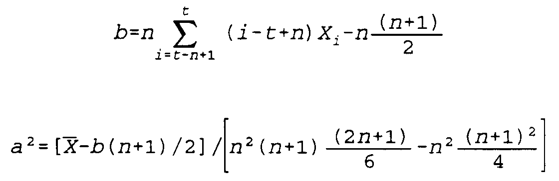

- The Sales Forecasting and
Planning Module 132 contains all the models and routines that are used to generate forecasts. These models and routines are used in theDemand Management Frame 130 for Bottom-up, Top-down forecasting, for the analysis of sales promotions and to estimate forecast accuracy. TheSFP Module 132 is also used in theVMR Frame 250. - The models and routines of
SFP 132 fall into three categories: generic models common to the manufacturing and repair environments; models specific to the manufacturing environment; and models specific to the repair environment. -
- Objective: Develop top-down and bottom-up sales forecasts.
- Scope: Products and selected customers.
- Features: Statistical forecast based on historical sales; Statistical forecast based on point-of-sale data if warranted; Customer provided forecast and orientations; and Reconciliation tools to support expert judgment such as exception flags and sanity checks.
- Three types of generic models are common to the manufacturing and repair environments. The first type consists of the various statistical forecasting models that can be used to forecast any time series (demand or consolidated requirement). The second type concerns the estimation of seasonality factors based on the same approach in both the repair and the manufacturing environments. The third type of model relates to forecast accuracy estimation.
- The objective of the Statistical models is to generate a forecast based on the projection of some historical characteristics of the time series. These models can be applied to any time series in the context of demand characterization, bottom-up, top-down forecasts and VMR.
- Below we discuss the following models: Moving average; Linear trend; Exponential smoothing; Holt-Winters model; Winter's method; Regression based forecasting model; and Autoregressive/moving average model (Box Jenkins).
- This conventional model is appropriate when the dependent variable is assumed to fluctuate around a constant (stationary) average value, i.e.:

- Time series data to be forecasted (for example POS or shipment)
- Window n: number of periods to be considered for averaging.
- Future forecasts and their variances.
-

Estimate
-

-

- This conventional model is appropriate when the dependent (forecastable) variable is assumed to fluctuate around a trend line, specified as a linear formulation of time, i.e.

- Time series data to be forecasted (for example POS or shipment) window n.
- Future forecasts and their variances.
- Select appropriate time period for trend estimation (the "window" of n periods).
-

-

-

- This conventional model is appropriate when the dependent variable is assumed to fluctuate around a constant (stationary) average value, i.e.:


- Time series data to be forecasted (for example POS or shipment)
- Smoothing parameter α
- Future forecasts and their variances.
- Initiate F1 as D0.

-

-

- This conventional model is also appropriate when the dependent (forecastable) variable is assumed to fluctuate around a linear trend line, i.e. when Xt is specified by:

- Time Series Data to be forecasted (for example POS or shipment).
-
Smoothing parameters 1>α≥β>0. - Future forecasts and their variances.
- Initial So and Go, intercept and slope of trend line.
Update recursively


-

- This conventional model is appropriate when the dependent (forecastable) variable is assumed to fluctuate around a linear trend line modulated by seasonality factors, i.e.


- Time Series Data to be forecasted (for example POS- or shipment).
- Season length N.
- Smoothing factors, α, β and γ.
- Future forecasts and their variances.
-
- Step 1: (Initialization). Use first two seasons (periods - 2N+1, -2N+2,...,0) to initialize values:
- 1a: Calculate sample means for two separate seasons of data.
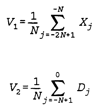
- 1b: Define G0 = (V2 - V1)/N as the initial slope estimate.
- 1c: Set S0 = V2 + G0 (N-1)/2, as an estimate of the value of the series at time t=0.
- 1d: Compute initial estimates of seasonal factors; these are obtained by dividing each of the initial observations by the corresponding point on the line connecting V1 and V2, i.e., compute:

- 1e: Average seasonal factors as computed for the two seasons

- 1f: Normalize seasonal factors:
- 1a: Calculate sample means for two separate seasons of data.
-


- Step 3: Create forward forecast in period t for period t+τ:

- In this conventional model, it is assumed that the forecastable variable X is determined by m(≥1) exogenously measurable (forecastable) variables Z(1), Z(2),...Z(3) as follows:

- Time series for {Xt} and all explanatory variables {Z(1), Z(2),...,Z(m)} For example market share, total market value, installed base, GNP, etc.
- Time series data to be forecasted (for example POS or shipment)
- Estimates of coefficients a, b1, b2,...,bm as well as σ2.
- Forecast for future value of X, on the basis of estimated future values of Z(1), Z(2),...,Z(m).
- Use of standard multiple regression method.
- In this category of models, it is assumed that the forecastable variable {Xt} exhibits an autocorrelated structure. The most general model of this type is specified as an ARMA (p,q)
model, i.e.

- Time series data to be forecasted (for example POS or shipment).
- Identification of optimal values of p and q.
- estimates of coefficients β 1,...,βp and γ 1,...,γq as well as σ2.
- Forecast of future value.
- Standard Box-Jenkins Algorithm and Process with forecasted value computed as follows:

- To estimate for each time bucket (quarter, month, week) its percentage of the yearly volume.
- Historic data by aggregated at the same level as the seasonality
- POS
- Shipment
- Total market volume, etc.
- Seasonality factors for each time bucket.
- Compute for each time bucket the proportion of the yearly volume it represents.
- To estimate the accuracy of the various types of forecasts. Measures of forecast accuracy are used in various contexts.
- It is a proxy measure for the variance of the forecast when this one cannot directly be computed. Forecast variance is used in several inventory and safety stock calculations.
- Forecast error measures can also be used to identified those products and customers for which demand patterns are particularly unstable and thus require special attention.
- To compute forecast error for the forecast produced n periods ahead.
- Actual Sales
- n periods ahead Sales Forecast (BU, TP, etc.).
- Average Absolute Error as of percentage
- Mean Square Error
- Table of forecast accuracy as function of n
- Compute the percentage difference between the forecasted and actual sales.
Compute average absolute error and mean square forecast error. - To generate the list of the products or customers for which the forecast error was greater that a predetermined forecast error threshold.
- Average Absolute Error
- Mean Square Error
- Forecast error threshold
- Rank list in decreasing order of Average Absolute Error or Mean Square Error
- Exception list: ordered list of products for which the forecast error was higher than the threshold
- The particular aspects of the manufacturing environment call for specific models in the area of forecasting and planning. In particular a forecast approach that specifically models the ordering pattern of retailers based on their replenishment policy and level of sale to the final consumer is considered. Approaches for the modeling of sales promotions are also proposed.
- This discussion describes an algorithm to compute bottom-up forecasts designed so as to result in the best available point estimates of sales as well as a characterization of the degree of uncertainty surrounding these estimates. The system develops forecasts for each account, each model and each time-period. These are subsequently aggregated over all accounts.
- The analysis starts with a characterization of the account's anticipated sales pattern for a given model. Its order to the manufacturer are obtained as derivatives of this sales pattern, assuming that a specific systematic replenishment policy is followed by the account. The prevalence of a systematic replenishment policy (in the absence of capacity problems) is an important assumption but one which we have verified in our analysis of real retailer's behavorior.
- Previous investigations of point-of-sales data have established that the accounts' sales pattern is much more predictable and regular than the normal order stream. It is therefore appropriate to start the forecasting process with a characterization of the account's sales pattern. Moreover, we envision that the inputs to the system be provided by the retailer in cooperation with or as a result of monthly meetings with account representatives (buyers, logistics managers). The account representatives are clearly more familiar with their sales pattern than the resulting order stream to their supplier; their estimates for future orders are clearly driven by their anticipation of future sales.
- The need to characterize the uncertainty of the manufacturer's model sales stems primarily from the fact that this characterization is to be used as the foundation for inventory planning, i.e. the determination of the so-called I-line or lower bounds for the I-line required to assure customer service levels which are compatible with the manufacturer's Quick Response targets.
- To assess minimum inventory requirements one needs to characterize cumulative sales over time rather than or in addition to sales per month. Extreme care needs to be exercised in aggregating sales over consecutive months since these are highly correlated. Thus, a straightforward convolution of orders in consecutive months would lead to serious underestimates of the variability of cumulative orders and hence to the determination of inappropriately low safety stocks (minimum inventory levels), exposing the manufacturer to undesirable frequent stockouts. These would result in inappropriate customer service, loss of market share and last but not least, a continuation of the vicious cycle preventing the manufacturer from establishing reliable forecasts in the first place.
- Our approach provides an exact characterization of the statistical distribution of cumulative sales based on a given characterization of the underlying sales pattern.
- The calculus used to characterize the distributions of account orders and aggregate orders is based on simple but rigorous probability calculus.
- The system is intuitive and fully transparent to all users. Below we give a brief outline of the inputs required by the system and the user interfaces which we envision developing to provide the user with various types of background information to facilitate the task of specifying forecast inputs.
- The calculus used to derive all order and aggregate order distributions is explained.
- The user will be responsible for entering forecasts for specific account/model combinations under his/her responsibility. For any given account/model combination, forecasts are to be provided for the next 12 months on a rolling horizon basis. The user will be confronted with a main menu permitting a choice between: (I) whether to provide estimates of the accounts' sales (I1) or orders (I2); and (II) whether to provide estimates of monthly total sales (orders) (II1) or to provide separate estimates (II2) for
- (a) regular sales activities, and
- (b) Promotional activities
- We will strongly encourage LAMs to opt for
- (1) providing estimates for sales, and
- (2) providing separate estimates for regular and promotional sales
- If option (I2) is chosen, the calculations described below will be circumvented and by default orders in consecutive months will be treated as independent. (This may result in important distortions as explained in the introduction but is unavoidable under this option; the user cannot be expected to estimate the intertemporal correlation pattern. It is conceivable that an "average" correlation factor may be inferred from historical orders.)
- All accounts managed by the three LAMs whom we have interviewed follow or would like to follow a simple replenishment policy of the following type: (a) the model's inventory position is reviewed periodically (e.g. once a week, once in two weeks, once a month); and (b) at review epochs the account places an order to increase the model's inventory position to a target level of a given number of weeks of future expected demands (e.g. 6 weeks, 8 weeks) unless the current inventory position is already above this target level in which case no order is placed.
- The formulae below are based on this type of replenishment policy which is characterized by two parameters only (the review period and the target order-up to level in weeks). This policy structure is easy to use and efficient from more than one point-of-view. However, it will be easy to make appropriate modifications should it become apparent that other types of replenishment policies are used by some accounts.
-
- st =
- sales in period t (random variable)
- µt =
- E st
- W =
- number of periods of future demands to which the inventory position is to be increased every time an order is placed.
- St min = minimum sales for period t
- St max = maximum sales for period t
- St most =most likely sales volume for period t
-
- ot =
- order in period t

- os =
- cumulative orders in
periods 1,...,t - IPt =
- inventory position at end of period t after placing an order (= inventory on hand + outstanding orders)
- Tt =
- target order-up to level at end of week

- The distribution of the IPt - variables can be computed recursively. Observe the IPt-1 and st are independent of each other.

- Hence,

- Hence,


The distributions of cumulative orders, i.e. the (0t) - distribution can be computed recursively as well but only by computing the joint distribution of 0t-1 and IPt-1: -
Case 1 Let k'>k:
- Case 2 k'=k:


- To assess the total impact on sales of past promotions.
- Promotions perturb the regular pattern of sales and various types of promotional activities influence the sales volumes according to rather different patterns. The objective of the model is therefore to assess the pattern of the impact of the promotion over time.
- Times series of sales.
- Time period of the promotion.
- Class of the promotion.
- Type of the promotion.
- Intensity of the promotion.
- Overall impact of the promotion
- Profile of the impact over time.
- The model is based on the use of time series models. First, an analysis is applied to a "censored" time series of sales volumes, in which all promotion (and after promotion) periods have been eliminated. One of several basic time series models is applied to identify trend factors, seasonality indices and/or auto correlation structures.These basic time series models include exponential smoothing (weighted) moving averages, Winters' model, Box-Jenkins models. The following Modified Winters' Procedure uses the demand (POS or shipment) data to remove seasonality and trend effects.
Select time series model for estimation of demand for non-promotion periods.
Initial Estimation of Level (including trend) at each Historical Period.
Calculate the moving average of seasons, with each season having period P. If P is an even number, take the average of two consecutive moving averages to let the estimate centered on the time period. - Divide the actual demand by the centered moving average to obtain the estimate seasonal factor. Dampen the random effects by taking averages for similar periods in different years. Then, normalize the estimate seasonal factors that totals to P. Using the normalized seasonal factors remove the seasonality effects from the demand data.
- Using the regression equation algorithm specified in the
MDA 134 module, find the regression parameters for level and trend coefficients to fit the regression line. Using the regression coefficients remove the trend effects from the demand data.
After an appropriate time series model has been selected for all non-promotion periods, interpolate base-line sales volumes in the promotion periods which would have arisen in the absence of the special promotion activities.
Calculate the ratios of the actual sales volumes during the promotion periods and the calculated "base line" values, for each promotion period separately. This defines the impact curve of the promotion.
Aggregate the impact curves pertaining to different promotion periods of a given type into a single curve using standard curve fitting techniques. - The resulting impact factors for each of the periods belonging to and following after a promotion interval can now be used in future forecasting efforts.
- To estimate the impact of a future promotion
- Time period of the promotion
- Class of the promotion
- Type of the promotion
- Intensity of the promotion
- Estimated overall impact of the promotion
- Estimated profile of the impact over time.
- Search promotion calendar for past promotions with similar characteristics.
Assess impact of the planned promotion based on computed effect of similar past promotions.
Identify generic profile of promotion impact corresponding to the planned promotion.
Compute estimated profile of the planned promotion by combining estimated total impact and generic profile. - This analysis includes the following three types of promotional activities: price promotions, where the item price is reduced by a given percentage for a limited period of time (e.g. 1-2 weeks); promotions via feature advertisements; and promotions via special store displays.
- The characterization of the impact of promotional activities is to be used as the basis of the statistical forecasting procedures in the Forecasting module of our
DSS 10. It will also be invoked as guiding information in the bottom-up forecasting procedure. - The sales promotion activities perturb the regular sales pattern in the commercial setting. Correspondingly, special events such as scheduled exercise in the defense application will also significantly change the usage of parts. Therefore, the models developed for analyzing the effects of sales promotions will also be applicable in understanding the effects of the special events in the defense setting. In the following section we employ commercial terminology for ease of explanation, while the models are equally applicable to both the defense and commercial applications.
- It is both intuitive and extensively substantiated by several statistical studies in the conventional marketing literature (see e.g., Blattberg and Naslin (1993)) that the various types of promotional activities influence the sales volumes according to rather different patterns. Price promotions typically result in a significant increase in the sales volume during the course of the promotion period. The increase in the sales volume is due to:
- a. consumers increasing their normal purchase quantities to take advantage of the temporary price discounts;
- b. consumers making a purchase during the promotion period who otherwise would have waited until a future point in time;
- c. consumers being enticed into a purchase who otherwise would have opted for a different brand or who otherwise would not be in the market for this item.
- Figure 31 displays a typical pattern for the percentage increases over time, resulting from a price promotion. As mentioned, the percentage increase is positive during the promotion period; the magnitude of the impact first increases and then decreases. The promotion period may be followed by an interval of time with a negative impact; the magnitude of the decline first increases and then decreases. See Lewandowski (1985) for more details.
- The impact of promotions via feature advertisements or special in-store displays may exhibit a similar pattern (as in figure 18); alternatively the impact of these types of promotions may be confined to the promotion period itself.
- Our menu of regression equations consists of variants of the following basic equation used in Blattberg and Wisniewski (1988) and with minor changes in Wittink et al. (1987).
Let: - Sit = Weekly retail sales for item i at time t,
- Rit = The regular (shelf) price of item i at time t,
- Pit = The observed price (actually paid by the consumer) for item i at time t,
- Dit = The deal discount for item i at time t ((Rit-Pit)/Rit),
- CPjt = The price of a competitive item j at time t with j not equal to i,
- Xit = A dummy variable which equals 1 if a display is run for item i at time t,
- Yit = A dummy variable which equals 1 if a feature ad is run for item i at time t,
- Lit = A variable representing deal decay, equaling kj-1 with j being the time since the beginning of the deal and 0<k<1,
- Ult =1 if period t arises l periods after the beginning of the last promotion period,
- l=1,K, u

- An alternative approach to analyze retailer promotions is based on the use of time series models. First, an analysis is applied to a "censored" time series of sales volumes, in which all promotion (and after promotion) periods have been eliminated. One of several basic time series models is applied to identify trend factors, seasonality indices and/or auto condition structures. These basic time series models include exponential smoothing (weighted) moving averages, Winters' model, Box-Jenkins models. The following Modified Winters' Procedure uses the demand (POS or shipment) data to remove seasonality and trend effects.
-
Step 1. Initial Estimation of Level (including trend) at each Historical Period.
Calculate the moving average of seasons, with each season having period P. If P is an even number, take the average of two consecutive moving averages to let the estimate centered on the time period. -
Step 2. Estimate Seasonal Factors.
Divide the actual demand by the centered moving average to obtain the estimate seasonal factor. Dampen the random effects by taking averages for similar periods in different years. Then, normalize the estimate seasonal factors that totals to P. Using the normalized seasonal factors remove the seasonality effects from the demand data. -
Step 3. Estimate Level and Trend Terms.
Using the regression equation algorithm specified elsewhere herein, find the regression parameters for level and trend coefficients to fit the regression line. Using the regression coefficients remove the trend effects from the demand data. - After an appropriate time series model has been selected for all non-promotion periods, one can interpolate the so-called base-line sales volumes in the promotion periods which would have arisen in the absence of the special promotion activities. By calculating the ratios of the actual sales volumes during the promotion periods and the calculated "base line" values, one constructs an impact-curve as in figure 31 for each promotion period separately. The impact curves pertaining to different promotion periods of a given type can next be aggregated into a single curve using standard curve fitting techniques, see figure 32. The resulting impact factors for each of the periods belonging to and following after a promotion interval can now be used in future forecasting efforts, as guided by our Forecasting Module. This approach follows that of Abraham and Lodish (1992) who have successfully adopted the methodologies in their earlier PROMOTER system to analyze retailer promotions. The PROMOTER model has four primary steps: (1) adjustment of the data for trend, seasonality, (2) elimination of data points influenced by promotion, (3) extrapolation of data points not influenced by promotion into promotion period, and (4) computation of promotion effect as the difference between this baseline and actual sales.

- Equipment consists of modules that are composed of reparable items, and repairable items are made of components.
Requirement: failure of an equipment.
Consolidation policy: the policy of replacing the defective reparable item of a failed module with a good reparable item of an already defective module and reinstalling into the equipment.
Defective ratio: ratio of number of defective reparable item to the total number of reparable items in a module.
Target level: maximum defective ratio acceptable before a module can be sent back from the equipment location to the repair depot. The target level is one of the two parameters of the consolidation policy.
Raw requirements (pre-consolidation requirements): total requirements generated by all equipment at the equipment location
Consolidated requirements (post-consolidation requirements): requirements for equipment after consolidation policy is applied to raw equipment requirements (number of modules sent to repair depot for repair from the equipment location)
Raw Requirements Estimation (for Bottom-up estimation) - To estimate raw requirements for all equipment located at a particular equipment location based on the planned activity (usage) schedules of the equipment.
- Equipment located at the equipment location.
- Activity schedules for all the equipment at the equipment location such as:
- equipment upgrade/maintenance schedules (preventive and breakdown maintenance schedules)
- activities (i.e., operation time, number of setups, cumulative operation time)
- planned activity schedules for all equipment at the equipment location
- Estimations of the raw requirements for each equipment at the equipment location
- Establish relationships between raw requirements and activities of the equipment based on analysis of graphs, etc.
Analyze the effects of activities on requirements using regression or time-series models
Estimate raw requirements for each equipment given the equipment's planned activity schedule by the models used above.
Consolidated Requirements Estimation (for Bottom-up estimation) - To estimate consolidated requirements for all equipment located at an equipment location based on the estimated raw requirements
- Estimated raw requirements for each equipment at the equipment location and the time of requirement
- Batching parameter for the batching policy of the equipment location
- Consolidation policy (target level and the search rule)
- Inventory positions at the equipment location for modules and reparable items
- Performance measures: stock level, service level (availability of equipment), repair cost associated with repair at equipment locations and the repair depot
- Estimates of consolidated requirements for all equipment at an equipment location
- Values of performance measures
- Search under consolidation policy
Identify repairable items to be sent to repair depot under batching policy of the equipment location - A consolidation policy consists of two elements: a search rule for selecting the defective repairable item to be consolidated, and a target level, that is the maximum defective ratio acceptable before a module can be sent back from the equipment location to the repair depot.
- Given a newly failed module of type I with a defective reparable item of type j, the consolidation policy defines which reparable item should be chosen out of which module to perform the consolidation. The chosen repairable item should already be part of a module with at least one defective reparable item but containing a good component of type j. The search rule select the reparable item for consolidation among all such defective modules. The following search rules are considered:
- Carry out the search for defective modules of type I only. Sort the defective modules of type I in decreasing order of the defective ratio and starting from the top of the list, select the first module that has a good component j in it, if one exists. If not, sort all the other defective modules in decreasing order of the defective ratio and starting from the top of the list, select the first module that has a good reparable item j in it, if one exists. If not, (consolidation cannot take place) replace the failed module I with a good one, if one is available at the equipment location. If not, equipment becomes unavailable until either a consolidation or a replacement can be made.
- Determine all module types for which stocks of good items at the equipment location are below a threshold value. Sort the defective modules of all such types in decreasing order of the defective ratio and starting from the top of the list, select the first module that has a good reparable item j, if one exists. If not, sort all the other defective modules in decreasing order of the defective ratio and starting from the top of the list, select the first module that has a good reparable item j, if one exists. If not, (consolidation cannot take place) replace the failed module of type I with a good module of type I, if a good one is available at the equipment location. If not, the equipment becomes unavailable until either a consolidation or a replacement can be made.
- Sort the defective modules of all types in decreasing order of the defective ratio and starting from the top of the list, select the first module that has a good reparable item j in it, if one exists. If not, (consolidation cannot take place) replace the failed module of type I with a good one, if one is available at the equipment location. If not, equipment becomes unavailable until either a consolidation or a replacement can be made.
- The batching policy is defined by the size of a batch, TH1, (TH1 can be equal to 1). The inventory policy is in the form of: count the number of defective modules with defective ratio greater than the target level. If this number is greater than TH1, then send TH1 units of repairable items to the repair shop else wait until this condition is satisfied.
- To estimate consolidated requirements for all equipment located at a particular equipment location based on historical data
- Time series of consolidated requirements for each equipment locations.
- Estimates of consolidated requirements for all equipment at an equipment location
- Use a conventional Kalman filter based algorithm and conventional statistical forecasting methods to estimate consolidated requirement for the equipment
- To determine a repair plan based on aggregate repair plan, and repair constraints (resource capacities and key component availability)
- Aggregate repair plan
- Available resource capacities and degree of flexibility to change resource capacities
- Key component availability (projected inventory positions, supplier and lead time information, inventory replenishment policy)
- Repair plan for the repair shop that is feasible with respect to the repair constraints (capacity and key component availability).
- Objective: Decide where to stock, how much and when to replenish in (hybrid) made-to-stock/made-to-order environment.
Scope: Single and dual echelon.
Features:
Single and dual echelon inventory models for how much and when to replenish stocking points. Cost vs. service trade offs to determine where to stock.
Deployment.
Models specific to manufacturing environment - This module contains a collection of finished goods' inventory models enabling the selection and evaluation of inventory policies. The module returns an I- and P- line extended to a given horizon (of T periods) beyond the current period. At this stage, all of the models represent settings where any given item is distributed to the customers from a single location.
- Forecasts of mean demands per item, per period (S' line); standard deviations of demands per period per item (σ' line); mean production lead times for each period per item (L' line); standard deviations of lead times for each period, per item (τ' line).
- Inventory (I) line
- Production (P') line
- Inventory strategies
Models are classified as follows: MI. Models with Non-Lumpy Demand; and MII. Models with Lumpy Demand. Lumpy demands refers to settings where demands are sporadic or experience extreme variability. The demand process for a given item will be classified as lumpy if the percentage of zero demand periods or the coefficient of variation of the demands is above pre-specified critical levels. - Within the category MI we next differentiate between: MI.1 Models managing inventories or on an item-by-item basis; and MI.2 Multi-item models with joint capacity constraints.
- The choice between these two categories depends on whether or not important interdependencies prevail between the items (in the form of joint capacity constraints or joint cost structures). Within each of the subcategories MI.1 and MI.2, different models can be selected based on the extent to which policy parameters are to be pre-specified by the user or computed based on an appropriate tradeoff between cost and service measures.
- As mentioned above, in this category inventories are managed on an item-by-item basis. Different models need to be invoked dependent upon the extent to which policy parameters are to be specified by the user. Alternatively, the models to be used can be determined endogenously based on an appropriate tradeoff analysis or optimization of various cost and service measures.
- In this model, the user specifies an order-up-to or base-stock level as a given number of weeks of inventory. Based on this inventory policy, the model projects out an I' and P' line for a scenario in which the forecasted mean demands are realized.
- The desired base-stock level for each period
- nt = number of periods of future forecasted demands in which the inventory position is to be increased at the beginning of period t, if below
-
- Step 1: Compute bt = St + St+1 +...+ Snt. (If nt is specified as a fractional value, bt equals:
bt = St + St+1+...+ Snt + (nt -
 nt
nt ) S
) S nt
nt )
)
- Step 2: Project I' and P' line. Let:
- Ib = inventory position (inventory level plus outstanding orders) before ordering at beginning of
period 1. - Pt = production volume ordered at beginning of period t.
- It+1 = max (bt, It) + Pt - St
- Pt+1 = max (bt+1 - It+1 ; 0)
- Ib = inventory position (inventory level plus outstanding orders) before ordering at beginning of
- Step 3: Evaluation of various service and cost measures.
- a) e.g., expected average inventory level,
- b) probability of stock-out,
- c) fill rate or percentage of demands satisfied from stock,
- d) number of setups,
- e) average backlog sizes.
- In this model, a policy is computed which minimizes the expected value of the aggregate of all relevant cost components, i.e. 1) setup costs; 2) inventory carrying costs; and 3) backlogging costs. The model is appropriate in settings where stock-outs are fully backlogged and where the inventory carrying and backlogging costs are proportional with the inventory levels and backlog sizes.
- Holding cost rates per item per period (h' line)
- Backlogging cost rate per items per period (p' line)
- Variable production cost rate per item per period (c' line)
-
- Step 1: Load S' (Sales), σ' (Standard deviation), L' (Lead times), τ' (Standard deviations of lead times), K' (setup costs), h' (Holding cost rates), p' (backlogging cost rates), c' (variable production cost rates);
- Step 2: Fit appropriate demand distribution to S', σ' lines.
Fit appropriate lead time distributions to L' and τ' lines. - Step 3: Solve for time-phased optimal (s,Q) policy. Such a policy has for each period t = 1,...,T, two critical levels st and Qt such that whenever beginning inventory position It<st an order is placed for (st+Qt - It) units. Parameters (st, Qt) are computed from the following recursion.
Let:- Vt(I) = expected minimum costs in periods t, t+1,...,T given that period t starts with an inventory position of I units.
- Gt(y) = expected (inventory carrying and backlogging) costs associated with period t. (This function uses the lead time and demand distributions computed in
Step 2 as well as the h' and p' lines.) - Dt = demand in period t.

Output:
For all t = 1,...,T;- xt*(I) = optimal order quantity at the beginning of period t, when inventory position = I.
- Step 4: Create I' and P' lines.
I1 is known; set P1 = production lot initiated inperiod 1 equal to X*1 (I). Then project recursively for t = 1,...,T- It+1 = It + x*t (It) - St
- Pt+1 = x*t+1 (It+1)
- Step 5: Evaluation of various cost and service measures, as in
Step 2 of model M1.1. - In this category of models the inventory policy minimizes expected setup and holding costs subject to user specified service level constraints. The user may choose between the two types of conventional service measures.
-
Type 1 Service Constraints:
Maximum permitted probability of a stock-out during lead-time following potential order at beginning of a given period. Let:- αt= maximum permitted likelihood of stock-out during lead-time following potential order at beginning of period t.
-
Type 2 Service Constraints:
Minimum acceptable fill rate during lead time following a potential order at beginning of period. Fill rate is defined as the percentage of demand satisfied from stock.
Let:- βt= minimum acceptable fill rate during lead time following a potential order at beginning of period t.
Type 1 or Type 2) as opposed to explicit stock-out or backlogging costs. - holding cost rates per item per period (h' line)
- maximum permitted stock-out probabilities per item per period (α' line), or minimum acceptable fill rates per item per period (β' line)
-
- Step 1: Load S' (Sales), σ' (standard deviations), L' (lead-times), K' (setup costs), h' (holding cost rates), c' (variable production cost rates), α (service level type 1) or β' (service level type 2). (Lead-times are specified either as constants or via ranges with associated likelihood for each value in the range.)
- Step 2: Fit appropriate demand distribution to S', α' lines. Determine lead time demand distributions.
Let:- LDt = lead time demand for order placed at beginning of period t. If lead time demand distribution is chosen to be Normal (for example), then set its mean and variance as follows:

- Step 3: Compute minimum inventory positions after ordering St , via Reorder Point Algorithm, below:
- Step 4: Solve for time-phased optimal (s,Q) policy.
Let:- Vt (I) = expected minimum costs in periods t, t+1,...,T given that period t starts with an inventory position of I units.
- Gt(y) = expected inventory carrying and backlogging costs associated with period t.
- Dt = demand in period t.

for all t = 1,...,T;- x*t (I) = optimal order quantity at the beginning of period t, when inventory position = I.
- Step 4: Create I' and P' lines.
I1 is known; set P1 = production lot initiated inperiod 1 equal to x*1 (I). Then project recursively for t = 1,...,T- It+1 = It + x*t (It) - St
- Pt+1 = x*t+1 (It+1)
- Step 5: Evaluation of various cost and service measures, as in
Step 2 of model M1.1. - This category of models plans simultaneously for a complete family of items incorporating various joint capacity constraints. The model plans production quantities on the basis of estimated mean demands; however, minimum inventory levels are specified to satisfy user specified service constraints (of
Type 1 orType 2, see MI.1.3, above). The P' and I' line are in this case determined by the solution of an LP-model. The user specifies whether minimum inventory levels are to be determined on the basis ofType 1 orType 2 constraints. In addition, the user chooses among a number of possible objective functions (performance measures) to select among feasible plans. - LP formulation for I products (or product group) K resources (Key Component and/or Lines) sets and T periods
-
- Sit = Demand for product i at period t
- sit = Minimum amount of product i at the end of period t
- Ii0 = Initial inventory of product i at the beginning of the planning horizon
- ami = Units of resource m, among resources in set Sk, required per unit production/repair of product i
- cmt = Units of resource m which becomes available at period t (In case resource m is a key component, cm0 is the amount of it available at the beginning of the horizon under consideration.)
-
- Pit = Units of product i to produce in period t
- xmit = Units of product i to produce in period t using resource m in Sk
- Iit = Inventory of product i at the end of period t LP (A) Optimize:
OV1, OV2, OV3 or OV4 specified below:
subject to
- calculate the inventory levels,
(2.1) and (2.2) ensure that consumption does not exceed resource availability,
ensure inventory is no less than pre-specified levels and ensure that production/repair is non-negative. - If yes, a production plan : Pit for i = 1,2,...,I and t = 1,2,...,T the corresponding inventory levels : Iit for i = 1,2,...,I and t = 1,2,...,T and remaining resources : slacks in (2.1) and (2.2).
- If no, display sources of infeasibility : surpluses in (2.1) and (2.2).
- OV1: Maximize maximum slack in resource constraints (2.1) and (2.2)
- OV2: (Balance Workload).
min Σ [ ami xmit/cmt ] - OV3: Minimize variable production and holding costs
min Σ [ cit Pit + hitIit] - OV4: Minimize maximum inventory in weeks
min maxit [ Iit/Sit ] -
- Step 1: Load S' (sales), σ' (standard deviations), L' (lead times), h' (holding cost rates), c' (variable production cost rates), τ' (standard deviations of lead times); resource utilization matrix [ami] capacity levels [Cmt].
- Step 2: Determine lead time distributions LDt, as in
Step 2 of MI.1.3. - Step 3: Compute minimum inventory positions after ordering s1 ,```,sT via Reorder Point Algorithm.
- Step 4: Solve above LP.
- Step 5: Identical to Step 5 of model MI1.1.
- Apply to lumpy demand. The lumpiness of demand is measured as proposed herein.
- This policy is suitable for low cost slow moving items with lumpy demand.
- S' line, cover period n.
- MAX level, inventory target.
Frames using these models include
PSI Planning Frame 160 (CF8)
VMR Frame 250 (CF19 and CF20) -
-
Step 1. Usemethod 1 to categorize lumpy demand -
Step 2. Determine 'n'; a worst case scenario would be to set 'n' as the replenishment lead-time. -
Step 3. Determine the maximum demand during period 'n' and set it as the inventory target, MAX. -
Step 4. Compute I' line:
Ijt-1+xjt-djt = Ijt for j = 1,2,...,J and t = 1,2,...T - This policy is suitable in cases where there are fairly expensive items that have lumpy demand.
- S' line
- Max level, inventory target
Frame using the model includes
PSI Planning Frame 160 -
-
Step 1. Usemethod 2 to categorize lumpy demand -
Step 2. Define expected deficit due to lumpiness as average amount that the quantity on hand is likely to fall before a replenishment order is placed. -
Step 3. Approximate the expected deficit (average period sales) as one-half of the beginning and ending quantity on hand between quantity-on-hand record updates. -
Step 4. Set ROP as safety stock plus demand during the lead-time and expected deficit. -
Step 5. Set the MAX level as the ROP quantity plus the order quantity less the expected deficit. -
Step 6. When the inventory level reaches the reorder point, the difference between the targeted quantity MAX and the quantity-on-hand is ordered.
Compute the I' line:
Ijt-1+xjt-djt = Ijt for j = 1,2,...,J and t = 1,2,...T
- To determine CSI level for each module type.
- repair shop repair time estimates
- consolidated requirements for equipment for the previous periods
- CSI levels for each repairable item type
- For each repairable item, set CSI level to CSImin, calculate the corresponding performance measures. Based on values of the performance measures and the estimated consolidated requirements, change the CSI level and repeat.
- Performance measures that can be considered for determining the CSI level for each repairable item are the total cost of repair (setup cost + repair cost), and the fill rate (service level) at the repair shop.
- CSI level for each repairable item must be greater than or equal to the value of CSImin, which is simply the sum of the requirements during repair time and a safety stock. CSImin ≥ E[requirements over all equipment locations during repair time of one unit] + safety stock where safety stock is a user defined parameter, based on past requirements.
- This process includes the objectives: (i). to estimate number of consolidated requirements for equipment triggering repair at the repair shop; (ii). given (i), to estimate number of repairable items requiring repair at the repair shop; and (iii). given (ii), to estimate aggregate repair requirements at the repair shop
- CSI levels
- consolidation policy target level
- Types and numbers of repairable items in each equipment
- BOM for each repairable item (to go to the component level)
- Final estimations of consolidated requirements for the equipment
- Final estimated repairable item requirements corresponding to the consolidated requirements for equipment
- Repair data for each repairable item (operation sequence and repair time estimates for each operation)
- Aggregate repair requirements at the repair shop
- Estimate number of consolidated requirements for equipment triggering repair at the repair shop
Estimate number of repairable items requiring repair at the repair shop
Estimate aggregate repair requirements at the repair shop
Generation of a feasible aggregate repair plan - To generate an aggregate repair plan based on aggregate repair requirements, and repair constraints (resource capacities and key component availability).
- Aggregate repair requirements
- Available resource capacities and degree of flexibility to change resource capacities
- Key component availability (projected inventory positions, supplier and lead time information, inventory replenishment policy)
- BOM for each repairable item family (to go to the component level)
- Aggregate repair plan for the repair shop that is feasible with respect to the repair constraints (capacity and key component availability)
- Check if aggregate repair requirements are feasible with respect to capacity constraints of the resources
If not, change capacity levels of flexible resources. If still infeasible, point out infeasibility and go back and move aggregate repair requirements forward or backward in time
Determine key component requirements and time of requirement from aggregate repair requirements
Check if aggregate repair requirements are feasible with respect to key component availability constraints
If not, point out infeasibility in terms of component availability. Change key component availability (if it can be changed) equipment based on the purchasing policies for the components. If still infeasible, go back and move aggregate repair requirements forward or backward in time until a feasible repair plan is generated - The
Aggregation Production Module 162 focuses on itsPSI Frame 160 application. The following two capacity checking models are identified and developed to support theModel Engine 20 requirements in thePSI Frame 160. - Objective: Facilitate the master production scheduling process.
Scope: Finished goods production in some aggregate view.
Features: Rough-cut capacity checking for finished goods; Major components (feeder plants) represented in constraints; and Ability to identify violated constraints. - In the Capacity Checking models, the problem of checking whether there is enough resources to satisfy requirements is formulated as Linear Programming Problems. These models are applicable to both the manufacturing and repairing environment in the PSI frame. The capacity checking models are presented in manufacturing terms these models also apply to the repair environment and are used in the context of the Requirement-Supply Reconciliation frame to assess the feasibility of a repair plan.
- Check whether there is a feasible production plan to satisfy given sales and safety stock requirements.
-
- I = The number of products to be considered.
- K = The number of resources (production lines and key components) sets.
- Sk = The set of resources.
- T = The planning horizon.
- Sit = Demand for product I at period t.
- ISSit = Safety stock of product I at the end of period t
- Ii0 = Initial inventory of product I at the beginning of the planning horizon.
- ami = Units of resource m, among resources in set Sk, required per unit production of product I.
- cmt = Units of resource m which becomes available at period t. (In case resource m is a key component, cm0 is the amount of it available at the beginning of the horizon under consideration.)
- If yes,
a production plan:
Pit for i = 1,2,...,I and t = 1,2,...,T
the corresponding inventory levels:
Iit for i = 1,2,...,I and t = 1,2,...,T
and remaining resources (slacks in constraints (3) and (4)):
Σs=0 to t cms - Σs=0 to t Σ i amixmis for each key component m and t = 1,2,...,T and cmt - Σ i amixmit for each production line m and t = 1,2,...,T.
If no, display sources of infeasibility (surpluses in constraint (3) and (4)):
Σs=0 to t Σ i amixmis - Σs=0 to t cms for each key component m and t = 1,2,...,T and Σ i amixmit - cmt for each production line m and t = 1,2,...,T. -
- Pit= Units of product I to produce at period t,
- xmit = Units of product I to produce at period t using resource m in set Sk,
- dit =Demand for product I during the period t,
- Iit = Inventory of product I at the end of period t.
- Minimize maximum production line utilization (smooth production line utilization):
Minimize z
subject to Σ I amixmit/cmt <= z for each line resource m and t = 1,2,...,T.
Minimize maximum inventory level:
Minimize z subject to Iit <= z for i = 1,2,...,I and t = 1,2,...,T.
Minimize total inventory level:
Minimize Σi Σt Iit
Minimize total inventory cost:
Minimize Σi Σt (hit Iit ++ pit Iit -)
subject to Iit = Iit +- Iit -, Iit +>= 0 and Iit - >=0 for I = 1,2,...,I and t = 1,2,...,T
where hit = cost per unit holding and - pit = cost per unit backlog of product I at the end of period t.
- Iit-1+Pit-dit=Iit for i = 1,2,...,I and t = 1,2,...,T.
Resource allocation
Σ m in Sk xmit =Pit for k= 1,2,..., K and t = 1,2,..., T.
Key component availability
Σs=0 to t Σ i amixmis<= Σs=0 to t cms for each key component m and t = 1,2,...,T.
Production line capacity
Σ i amixmit<=cmt for each production line m and t = 1,2,...,T.
Safety stock requirement
Iit>=ISSit for i= 1,2,...,I and t = 1,2,...,T.
Non-negative resource allocation
xmit>=0 for m in Sk, k= 1,2,..., K, i = 1,2,...,I and t = 1,2,...,T.
Capacity Checking Model
CCM1 : User selected objective function subject to the above constraints.
Frames using this model include PSI planning (CF13), VMR. (CF 20) - This LP formulation, with minor changes, is also applicable to a repair environment, where reparable items correspond to products, repair requirements for reparable items correspond to demands for products, and broken reparable items awaiting repair at the repair shop correspond to key components.
- For the repair environment, key component availability constraint (the fourth constraint) should be modified as in the following to represent broken reparable item availability at the repair shop :
4) Broken reparable item availability:
Σs=0 to t Σ m xmis<= Σs=0 to t cis for each repairable item i and t = 1,2,...,T. - Objective functions and the other constraints in a repair environment will be similar to those of a production environment, which are given above. The LP model for the repair environment will either produce a capacity feasible aggregate repair plan that satisfies the repair requirements generated by reparable item failures or display sources of infeasibility.
- Check whether a given production plan is feasible with respect to aggregate production capacity and key component availability.
-
- I = The number of products to be considered.
- K = The number of resources (production lines and key components) sets.
- Sk = The set of resources.
- T = The planning horizon.
- Pit= Units of product i to produce at period t.
- ami = Units of resource m, among resources in set Sk, required per unit production of product i.
- cmt = Units of resource m which becomes available at period t. (In case resource m is a key component, cm0 is the amount of it available at the beginning of the horizon under consideration.)
- If yes, display remaining resources (slacks in constraints (3) and (4)):
Σs=0 to t cms - Σs=0 to t Σ i amixmis for each key component m and t = 1,2,...,T and cmt - Σ i amixmit for each production line m and t = 1,2,...,T.
If no, display sources of infeasibility (surpluses in constraint (3) and (4)):
Σs=0 to t Σ i amixmis - Σs=0 to t cms for each key component m and t = 1,2,...,T and Σ i amixmit - cmt for each production line m and t = 1,2,...,T. -
- xmit = Units of product I to produce at period t using resource m in set Sk.
- CCM2 : Objective function 1) subject to constraints 2), 3), 4) and 6).

- This section describes the specifications of the various models used in the VMR modules. The description is divided into three main categories: (1) Inventory Requirements Setting Models, (2) Strategic Models, and (3) Operational Models. The notation for these models is introduced as necessary throughout this section.
- The models developed in this section are based on prior results in the professional literature as well as from other sources.
- Objective: Analyze contractual agreements with customers; and Decide on what to ship, in what quantities and when.
Scope: Selected products for selected customers.
Features:
Evaluate policy parameters such as bounds on customer inventories, target service level and delivery frequencies. Statistical forecast of retailers' sales (i.e. forecast of sales of PCEC's customers to their customers). Determine shipment requirements and delivery schedules.
Inventory Positioning: The Multi-Item, Two Echelon Model - This section presents two models; the first model describes an algorithm for the calculation of required echelon inventories. (Echelon inventory = inventory in transit from the plant to the DC + inventory on hand at the DC + inventory in transit from the DC to the stores + inventory on hand at the stores.) The second model estimates the expected level of service provided at a certain D.C, given a delivery quantity. Two important parameters used in both models are the expected value and standard deviation of the lead-time demand. These models compute the stock-out probability of today's delivery on the day of its arrival to the stores. This is based on the approximation that was developed as part of prior research on the Multi-Item, Two-Echelon production/inventory systems Setting Inventory Requirement: Model (R)
- This module computes the required echelon inventory levels (R' line) at the beginning of each review period over the whole planning horizon. Clearly, these requirements depend on the delivery frequency used (the requirements increase as the delivery becomes less frequent). Thus, the required inventory levels (R' line) are calculated separately for each one of the pre-specified delivery frequencies.
- Network structure.
- Demand forecast (means, standard deviations and dispersion factor).
- Required service levels (in terms of stock-out probability).
- Set of possible delivery frequencies.
- Lead-times from each plant to every DC it replenishes, and the average lead-times from every DC to the stores it supplies.
- Planning horizon specifications
- Required inventory lines (R' lines).
-
- t0 - beginning period of the planning horizon (assuming that 'today' is the beginning of period number 1).
- T - the length of the planning horizon.
- Rt f(i,j) - required inventory level, of product j at DC I, at the beginning of period t, when delivery frequency f is applied.
- αij - required service level for product j at DC I.
- µt ij - mean demand for product j at DC I during period t.
- σt ij - standard deviation of the demand for product j at DC I during period t.
- δt ij - demand dispersion rate for product j at DC I. The dispersion rate is defined as follows:

- Lij - Lead-time from the plant that produces product j to DC I.
- λij - Average lead-time from DC I. to its stores, for product j.
- Q - Set of 'quarters' into which the planning horizon is split. Each quarter is a continuous time interval consisting of one or more periods.
- Qq, ¦Qq¦ - Quarter number q and the number of periods in it (note that ).
- F - The set of all possible delivery frequencies. Each delivery frequency f is specified as the minimal number of periods between two consecutive delivery periods. The values f must be integral (for non-integral values, redefine the base period, e.g. half a week instead of a week).
- µt ij(m), σt ij(m) - The mean and standard deviation of the demand for product j at all stores supplied by DC I, over periods t until t+Lij++m (m≥0 is a parameter of these functions). The term t+Lij++m represents the expected time at which a delivery shipped from the plant at period t+m (next possible delivery time), arrives to the stores.
- For all product-DC couples (i,j)
For all frequencies f in F
time := 0
For all 'quarters' q in Q
For all periods t = 1 to ¦Qq¦
time := time + 1
// compute the time to next feasible delivery period,
t_del. //
t_del := f - [ ( t + f - 1 ) mod f ]
time_to_DC := t_del + Lij
time_to_stores := time_to_DC + lij
compute the values
(R.4) mean = α ·ij λ


End For (q)
End For (f)
End For (i,j)
Estimate Stock-out Probability for a Given Replenishment
Quantity: Model (OR1): - For a given replenishment quantity of product j, delivered from plant p(j) to DC I, this model estimates the expected projected stock-out probability. The stock-out probability is defined as the probability of shortage in at least one of the stores replenished by the DC The word "projected" refers to lead-time periods later, when goods are expected to reach the stores.
- In addition to the notation defined up to this point, we define:
- DELIV - delivery size.
- date - date of delivery.
- arr - (expected) arrival date of goods to stores
- Xij date - the echelon inventory level of product j in DC I, at (period) time date.
- Use formula (R.2), with t_del=1, to calculate the expected demand over the lead-time,


The projected stock-out probability can be approximated by:

- This module consists of a set of models tailored to support replenishment planning by integrating: (1) service level requirements; (2) limits on customers' inventory investments; (3) transportation costs; and (4) delivery frequency.
- Below is the input which is common to all of the models described in this particular discussion:
- Network Structure,
- Demand Forecast,
- Lead-times from each Plant to each DC and (an average) from each DC to its Stores,
- Planning Horizon Specifications
- Current Inventory Positions,
- Transportation Cost Structure and Trucks Volumes,
- Products' Volumes (for Transportation Cost Calculations),
Computing The Optimal Delivery Frequencies: Model (C1) - This model computes delivery frequencies from each plant to the DC it replenishes such as to minimize total transportation costs. The delivery frequencies are set such that given requirements on service levels are satisfied and such that constraints on average inventories are not violated.
- Inventory Requirements (R' Line, see Model R).
- Set of Possible Delivery Frequencies,
- Required Service Levels (in Terms of Stock-out Probabilities),
- Limits on Maximal Inventory Investments (in terms of Weeks of Demand),
- Delivery Frequencies,
- Estimated Level of Service,
- Estimated Transportation Costs,
- Estimated Inventory Levels,
- We use the same notation as in Model R (except for the notation for delivery frequencies) plus the following:
-
- i - DC index
- j - product (module) index
- p - plant index
- f - delivery frequency index
- s - index of line segment of transportation cost function (the cost structure is approximated by a piece-wise linear function)
- t - time index
- q - quarter index ()
-
- I - set of all DCs
- J - set of all products
- P - set of all plants
- F - set of possible delivery frequencies
- Ji - all products sold to DC i.
- Jp - all products produced in plant p.
-
- volip - total volume of a single truck
- cip - cost of full truck load (FTL)
- fixip - fixed cost of less than full truck load (LTL)
- τip,s - (right) end point of the s-th line segment (i.e., [τip,s-1 , ip,s] ) of the LTL cost function.
- rateip,s - transportation cost rate for volumes in segment s (i.e., in between τip,s-1 and τip,s), for LTL shipments.
- vj - volume of product j (for cost calculation purpose) - upper limit on the average number of weeks of inventory in DC i in quarter q.
-
- Xt ij - echelon inventory of product j at DC I (including outstanding orders) in the beginning of period t.
- St ij - delivery quantity of product j to DC I in period t.
- Fq ipf - an indicator set to 1 if in quarter q a delivery frequency f is followed for the replenishment of DC I by plant p. Otherwise it is set to zero.
- NFTt ip - number of full-truck-load sent to DC I from plant p during period t.
- LTLt ip - volume of LTL (zero if none) shipment sent to DC I from plant p during period t.
- Yt ip,s - total volume of LTL shipment that falls into line segment (cost rate category) number s. Note that .
- Zt ip,s - an indicator set to 1 if the LTL shipment size is larger than τip,s-1; i.e., segment s is partially or entirely covered. Note that Zt ip,s is always less or equal to Zt ip,s-1 .
- The following Mixed-Integer Linear Programming problem is solved:
Problem (C1):
Initialize inventory positions:
(C1.1)
(C1.2)
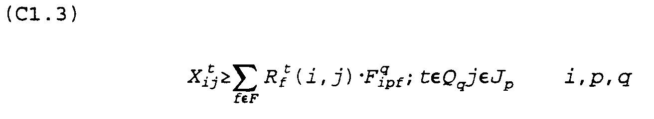


Computing Maximal Average Levels of Service: Model (C2) Objective: Given the delivery frequencies and limits on the average number of weeks of (echelon) inventories, this model calculates the maximal average service level that can be obtained. - Inventory Requirements (R' Line, see Model R)
- Delivery Frequencies
- Limits on Maximal Inventory Investments (in terms of Weeks of Demand)
- Estimated Level of Service
- Estimated Transportation Costs
- Estimated Inventory Levels
- We use the same notation as in Model C1 plus the following:
- αt ij - "projected" (i.e. "lead-time" periods after period t) level of service for product j in DC I at period t.
- Tip - a given set of periods in which replenishment (from plant p to DC I) is permitted.
- wij - values of objective coefficients (see discussion later)
- m - number of "segments" in the piece-wise linear function.
- θs - the s-th breakpoint of the piece-wise linear function (s=0,...,m); i.e. the s-th segment is given by [θs-1 , θs ].
- ∂s - the slope of the s-th segment of the piece-wise linear function (s=1,...,m).
- Zt j,s - the binary variables associated with this transformation.
- Yt j,s - the continuous variable associated with this transformation.
- The weights wij should be set such that

In case that some products have low service levels, the problem can be resolved with the addition of the following constraint

Minimizing Average DC Echelon Inventory Levels: Model (C3)
Objective: Given the delivery frequencies and required service levels, this model computes the minimal average number of weeks of inventories at each one of the DCs in every quarter. - Inventory Requirements (R' Line, see Model R)
- Delivery Frequencies
- Required Service Levels (in Terms of Stock-out Probabilities)
- Estimated Level of Service
- Estimated Transportation Costs
- Estimated Inventory Levels
- We use the same notation as in Model C2 plus the following:
- p(j) - the plant in which product j is produced,
- q(t) - the quarter to which period t belongs,
- Rt(i,j) - this is the inventory requirement as defined for Model R, but without the subscript f. It now refers to the given delivery frequency from plant p(j) to DC I in quarter q(t).
- AVGt i - the average echelon inventory level in terms of weeks of demand (for DC I in quarter q).
- For each DC I in I:
- Step 1: For each product j, j∈ Ji :
Solve the following problem:
S.T.
(C3.1) (C1.1) (single constraint)
(C3.2) (C1.2)
Beginning inventories must satisfy minimal requirements:
End For (j) - Step 2: For each q in Q
Calculate the value
End For (q) End For (I) - Given a delivery plan (i.e. the values St ij), this model computes the following operating values: (1) estimated inventory levels, (2) estimated levels of service, and (3) estimated transportation costs.
- Delivery Plan (St ij).
- Estimated Level of Service
- Estimated Transportation Costs
- Estimated Inventory Levels
-
- Pi - Set of all plants that replenish DC I.
- For each DC I in I:
- Step 1: Evaluate the expected (echelon) inventory positions at the beginning of each period via the equations (C1.1), (C1.2)
- Step 2: For each quarter q in Q
- 2.1 Evaluate the value AVGt i via (C3.4)
- 2.2 Evaluate the expected levels of service () via (C2.4).
- 2.3 Evaluate total transportation costs over the quarter (can be done by an external procedure) for each plant .
- This model checks whether a set of constrains (service levels, maximal echelon inventory levels and delivery frequencies) is compatible or not.
- Inventory Requirements (R' Line, see Model R)
- Set of Possible Delivery Frequencies
- Required Service Levels (in Terms of Stock-out Probabilities)
- Limits on Maximal Inventory Investments (in terms of Weeks of Demand)
- Feasibility (Yes or No)
- For each I in I:
- Step 1: For each plant p∈P:
Select the most frequent among the feasible delivery frequencies from plant p to DC I (this represent the less restrictive constraint).
For this delivery frequency, evaluate the inventory requirements Rt(i,j) by using Model R.
Calculate the values Xt ij as in Model C4.
End For (p)
- Step 2: For each q in Q
Evaluate the value AVGt i via (C3.4)
Check that
End For (q)
End For (I) - This model suggests both production and delivery schedules which minimizes total transportation costs and (in-plant) inventory holding costs. The plan is determined under service level constraints and constraints on average inventories at the DC (echelon) levels.
- Inventory Requirements (R' Line, see Model R)
- Set of Possible Delivery Frequencies
- Required Service Levels (in Terms of Stock-out Probabilities)
- Limits on Maximal Inventory Investments (in terms of Weeks of Demand)
- Delivery Frequencies
- Estimated Level of Service
- Estimated Transportation Costs
- Estimated Inventory Levels
- Estimated In-Plant Inventory Costs
- Proposed Production Plan
- We use the same notation defined up to this point plus the following:
-
- hj - holding cost, for unit of product j (in plant p(j)), per period.
- inv1 j - inventory of product j in plant (p(j)) at the beginning of the planning horizon.
- M - "big" number (see (C6.5)).
-
- I(j) - set of all DCs that carry product j.
-
- PRODt j - production batch size of product j in period t.
- INVt j - inventory of product j in plant p(j) at the beginning of period t.
- The following Mixed-Integer Linear Programming problem is solved:
Problem (C6):
(C6.1) (C1.1)
(C6.2) (C1.2)
Initialize levels of in-plant inventories:
beginning inventory = last period beginning inventory + production quantity in the last period - goods delivered during the last period:

See (C1.3):
(C6.9) (C1.6)
(C6.10) (C1.7)
(C6.11) (C1.8)
(C6.12) (C1.9)
(C6.13) (C1.10)
(C6.14) (C1.11)
(C6.15) (C1.12)
(C6.16) (C1.14)
(C6.17) (C1.15)
Options for Production Capacity Constraints:

- Similarly to (C6.18) and (C6.19), analogous sets of constraints can be constructed in order to express, for each plant: (1) limits on individual storage volumes, and (2) upper limits on total volume (value) of storage, respectively.
- In this section we describe a family of models, analogous to Models (C1)-(C3). The models are built to assist production and delivery planning for the short-term horizon. The major characteristics of these models are:
Rolling horizon planning: production and delivery plans are made frequently (even before the end of previous planning horizons), thus taking into advantage updated information about demands and production capacities.
High level of details: capacity constraints are more detailed so that the resulting plan will both be feasible and smoothly translated into production orders.
Flexibility in setting non-delivery periods: the user is allowed to specify periods in which delivery cannot be made. This replaces the requirement for following a certain delivery frequency. For instance, even if there is a certain guideline on delivery frequency, it can be relaxed at any (arbitrarily chosen) period. This reflects in added flexibility, which is especially important in cases of unexpected, high levels of demands (i.e. when deliveries must be made quickly). - The number of constraints (per period) is larger in these models, however, the planning horizon is usually much shorter than that of the strategic model. In addition, since we do not need to select certain delivery frequencies there is no need to incorporate the integer variables Fq ipf. This results in a significantly faster solution time.
- This model minimizes the total transportation and (inplant) inventory holding costs (see Model C6 for more details).
- The notation here is similar to that of Model C6 with the addition of the following:
-
- reqt ij - requirement for echelon inventory level of product j at DC I in period t, in order to maintain a certain level of "projected" level of service (see Model OR1 for further clarification). This minimal level depends on the delivery schedule, see Model R for explanation on how to calculate these values (very similar to the calculation of the values Rt f(i,j)).

- capt p(k) - the availability of resource k in plant p, in period t.
- λt j(k) - the amount of resource k required for a production of unit of product j in period t.
- storaget p(k) - maximal total volume/value (etc.) of inventory remaining at the end of period t in plant p.
- βt j(k) - the volume/value (etc.) of unit of product j in period t
- setupt j - setup cost to initiate a production batch of product j in period t.
-
- NoDelip - set of periods in which no delivery is allowed from plant p to DC I.
-
- PRODt j - production batch size of product j in period t.
- INVt j - inventory of product j in plant p(j) at the beginning of period t.
- SETt j - an integer variable indicating whether a setup is required in period t for product j.
- The following Mixed-Integer Linear Programming problem is solved:
(OP1):
(OP1.1) (C1.1)
(OP1.2) (C1.2)
(OP1.3) (C6.3)
(OP1.4) (C6.4)
Deliveries can be set to zero at any period the user chooses:

(OP1.8) (C1.6)
(OP1.9) (C1.7)
(OP1.10) (C1.8)
(OP1.11) (C1.9)
(OP1.12) (C1.10)
(OP1.13) (C1.11)
(OP1.14) (C1.12)
(OP1.15) (C1.14)
(OP1.16) (C1.15)
Production capacity constraints (see also Model (C6)):

The operational model can be extended so as to include setup costs (and/or setup times) as follows:
The term
Appropriate set of constraints should be added as well; for instance:
- This constraint is pertinent if product j requires a new setup in each period it is produced. (M is a "large" number.)

- The purpose of this model is similar to that of its long-term counterpart, Model (C2). In the same spirit of that model (C2), we change Model (OP1) as follows:
- (OP2):

(OP2.1) (OP1.1)
(OP2.2) (OP1.2)
(OP2.3) (OP1.3)
(OP2.4) (OP1.4)
(OP2.5) (OP1.5)
(OP2.6) (OP1.7)
(OP2.7) (C2'.4)
(OP2.8) (C2'.5)
(OP2.9) (C2'.6)
(OP2.10) (C2'.7)
(OP2.11) (C2'.8)
(OP2.12) (OP1.5)
(OP2.13) (OP1.17)
(OP2.14) (OP1.18) - Constraints (OP2.7)-(OP2.11) use the piece-wise linear approximation to the Standard-Normal cumulative distribution function (CDF), see below.
For explanation about the coefficients wij, see Model (C2)q i.
Note that in this case, in contrary to Model C2, the problem is not separable in I. This is due to the capacity and storage constraints (OP2.13) and (OP2.14), respectively. - This model is analogous to the long-term model, (C3).
We modify Model (OP1) as follows: -
- Step 1: solve the following problem:
(OP3):
(OP3.1) (OP1.1)
(OP3.2) (OP1.2)
(OP3.3) (OP1.3)
(OP3.4) (OP1.4)
(OP3.5) (OP1.5)
(OP3.6) (OP1.6)
(OP3.7) (OP1.17)
(OP3.8) (OP1.18) - Step 2: For each DC I:
Compute the values
- Determine which procurement policy should be used for which component.
- All components in planning bill of materials.
- Heuristic to identify the procurement policy to use for each component. The policies considered are: Just in Time; Bulk purchase, managed via stock policy, such as (s, S); and MRP calculus implying periodic purchase orders.
- Determine the number, location and capacity of distribution warehouses from a given set of potential locations.
- Distribution network excluding VMR arrangements.
- Use market demand projections to reengineer the existing distribution network.
- Global optimization of system-wide costs including inbound /outbound transportation, fixed and variable warehousing, and inventory carrying costs.
- In addition to the seven modules defined above, there is also a group of general purpose numerical routines that are not specific to any of the above seven modules. These routines are collected into a design element referred to as the Model Engine utilities 22, as shown in figure 35A. Examples of the Model Engine utilities 22 include generic linear programming solvers, and statistical analysis routines.
- In this section, we suggest few continuous. piece-wise linear approximations for the cumulative Standard Normal distribution curve. We use the following notation throughout:


- Consider an LP/MILP which minimizes a (linear) function of the decision variables X=(X1,...,XM,...,XN) and their piece-wise linear functions F1(X1), ...., FM(XM), M ≤ N. That is, an objective function of the type


- Let the function F:+→
 , be as follows:
- Ys - Is a continuous variable (Ys∈+) that represents the part of segment s "covered" by T , s=1,...,m ; that is,
(B.4)
- Is - Is a Binary variable (Is∈{0,1,2,...}) that indicates whether ) that indicates whether T covers any positive part of segment s; that is,


Ys (s=1,...,m) are the split of T into the segments.
Hence,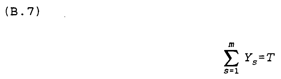
(B.8)
(B.9)

- This algorithm computes the statistical sample mean of a given time series for a given period of time.
The input for the routine is the time series , and time periods that the mean is computed over. The output is the unbiased sample mean quantity
- The algorithm computes the statistical sample standard deviation of a given time series for a given period of time.

The output is the unbiased sample standard deviation quantity σx. - The algorithm computes the moving averages for a given time series for a given period of time with specified averaging periods.


- The algorithm computes the seasonality factors for a given time series for a 12-month year period. The input for the routine is the time series, and time periods that the moving average is computed over (at least two seasonal cycles). The output is the seasonality factors.
- The algorithm computes the trend information for a given time series for a given period of time. The input for the routine is the time series, and time periods that the trend is computed over. The output is the trend value of the time series.
- There are several different methods to calculate the seasonality factors and the trend in a time series. The most popular ones include Winter's conventional linear and seasonal exponential smoothing, and (multiplicative) decomposition method developed by the U.S. Census Bureau, and its variant X-11 method).
- This algorithm computes the correlation coefficient for a given pair of time series with properly defined time periods (there might be certain shifts in time periods in the two time series).

- This conventional algorithm determines a curve with desirable shape to link a set of given points on a 2-dimensional space. The input for the routine is the set of given points, and the desired curve shape. The output is the curve that satisfies the required conditions.
- The algorithm computes the weighted sum of two time series.


- This algorithm computes the coefficient of variation for a given time series using unbiased statistical mean and standard deviation.

- This algorithm computes the goodness-of-fit (measure of accuracy) for a given pair of time series: one is the original time series and the other is the simulated one. The input for the routine is the pair of two time series, and corresponding time periods used to compute the goodness-of-fit for the two time series. The output is the goodness-of-fit (one measure of accuracy) for a given simulated method. The measure of accuracy can take one of the following forms (assume that X=Xt)1 n is the original time series, F=(Ft)1 n is the forecast time series and ei = Xi-Fi are the error terms):
Mean Error:


- This conventional algorithm computes the coefficients of a regression equation for a given set of time series. We will choose a standard computational routine to calculate these coefficients. The input to this routine is the set of time series. The output will be the calculated coefficients of the regression equation.
- A
Frame 16 is designed to integrate User Interfaces, models, analysis routines and data in order to address a set of related decision issues. The SupplyChain Frame Manager 24 constitutes the backbone of theDSS 10 through which the User Interfaces, the models in the modules and the data are connected. The SupplyFrame Chain Manager 24 facilitates the integration of the client side of the system, with which the user interacts, with the server side of the system where the modules and theDSS Database 12 reside. - The Supply
Chain Frame Manager 24 is responsible for two types of integration: System Integration and Functional Integration. The System Integrator 310 (see figure 34) is responsible to interpret the client's request, dispatch the request to the appropriate servers and to coordinate the computation load and data access. TheFunctional Integrator 312 provides the functionality associated with overall supply chain instead of individual frame. These functionalities include Supply Chain Configuration, Domain Management, user access or privilege administration and performance monitoring or simulation. - The
Frame Manager 24 is responsible for the client-server integration in theDSS 10. In this aspect, theFrame Manager 24 provides the linkage between theFrames 16,Model Engine 20 and theDSS Database 12; responds to the decision requests from the client programs by accessing the models and data; and maintains the "component objects" (e.g., object linking and embedding OLE objects) that share functionality betweendifferent Frames 16. Based on the decision requests, theFrame Manager 24 launches the appropriate object with the appropriate data, manages the requests from different clients for the same service and executes the appropriate server programs. The server programs execute the request, and return the results to theFrame Manager 24. TheFrame Manager 24 will interpret and return the results to theFrames 16. - The high level architecture of the
System Integrator 310 is shown in figure 35 and includes aClient Manager 320, aRequest Interpreter 322 and aServer Manager 324. - The architectural design of the
Frame Manager 24 reflects maximum flexibility and robustness of theDSS 10. The client side includes all theUser Interface 18 of each Decision Support Frame, such as Demand Management, Supply Management, etc. TheFrame Manager 24 includes two major pieces, theFunctional Integrator 312 and theSystem Integrator 310. Two other components running on the server side are Decision Support System Database (DSS Database 12) and theMathematical Model Engines 20. Theclient program 314 talks to theFrame Manager 24. TheFrame Manager 24 is the one responsible to call individual components running on the server to fulfill the client's request. - For example, a user is working on a PSI frame to develop production plan for a specific scenario. After deciding several key parameters, the user wants to check on the production capacity. The user makes this request from the User Interface 18 (click a button or select a menu item). The request is sent to the
Frame Manager 24. TheFrame Manager 24 interprets the request and determines that it needs to move the Capacity Checking Model to get the answer. (In a more general case, it may need to call more than one Model to accomplish the job.) Then theFrame Manager 24 determines whether a model Server already running and on which machine it is running. If there is one, it sends the capacity checking request, along with the necessary data, to that server. If there is no Server running at that time, theFrame Manager 24 will start up one on a selected machine and sends the request there. Sophisticated dispatching policies can be implemented at theFrame Manager 24 to balance the load or improve response times. After theModel Engine 20 finishes the job, it returns the result to theFrame Manager 24. TheFrame Manager 24 then synthesizes the result and returns the result to the client. - When the
Frame Manager 24 calls theModel Engine 20, it has two options in terms of passing the data. First, it can obtain the data from theDSS Database 12 and pass it to theModel Engine 20. This will be done when the amount of data that need to be sent to theModel Engine 20 is not very large. The advantage of this approach is that theparticular Model Engine 20 does not require the capability to accessDSS Database 12. But the data has to travel fromDSS Database 12 to FrameManager 24 and then fromFrame Manager 24 to theModel Engine 20. The second way to pass data to theModel Engine 20 is for theFrame Manager 24 to only pass the key information directly to theModel Engine 20. Then theModel Engine 20 accesses the data directly from theDSS Database 12 using the key information. This will be used when the amount of data needed by theModel Engine 20 is quite substantial, e.g. a situation of solving a Linear Programming model. The key information passed from theFrame Manager 24 to theModel Engine 20 will include the location of theDSS Database 12, among others. - The
Client 314 only interacts with theSystem Integrator 310 part of theFrame Manager 24. TheFunctional Integrator 312 part of theFrame Manager 24 provides the functionality through theSystem Integrator 310. The relationship between theFunctional Integrator 312 and theSystem Integrator 310 is logically the same as the relationship between theModel Engine 20 and theSystem Integrator 310. - The
System Integrator 310 in turn is composed of theClient Manager 320, theRequest Interpreter 322 and theServer Manager 324. TheClient Manager 320 manages and monitors the client connection. For example, it may disconnect a client if the client's machine is down or if the client is inactive for extended period of time. TheServer Manager 324 manages the server side connection. It is responsible to start up and shut down servers. It is also manages disparching. TheRequest Interpreter 322 is the one that the client directly interact with. It will parse the client request and generate request to the servers. It will consult with theServer Manager 324 before making connection to one specific server. - The high level object representation of the
system integrator 310 portion of theFrame Manager 24 is shown in figure 36 and the high level architecture is depicted in figure 37. The implementation documentation can be found in Appendix C. - The
Functional Integrator 312 enables the advanced user to define the supply chain configuration, manages user access and privileges, supports and enables the customization of theDSS 10, manages domains to support user defined data groupings, manages user definedScenarios 78 and ensures data consistency across theDSS 10, and dynamically monitors the impact of the user's decisions on the performance of the entire supply chain by using supply chain simulation. - The Supply
Chain Frame Manager 24 allows the advanced user to specify the configuration of the supply chain. The advanced-user will be able to specify the structural (static) elements of the supply chain. These include: Customers or Equipment; Products or Repair Items; Components; Production Resources or Repair Resources; For each of these structural elements, the advanced user will be able to define the various attributes such as; Names and the values of features; Group definitions; and Nodes and locations. - In addition, the advanced user will be able to define the inter-relationships between these structural elements. These interrelationships include: Distances, costs, and flow limits on the arcs between the various nodes of the network; Customer-Product-Resource (Equipment-Repair Item-Resource) relationship matrix; Bill of Material structure that relates components to products; and Production Matrix that relates production resources (repair resources) to products (repair items).
The data flow diagram associated with the SupplyChain Network Configurator 330 is shown in figure 38. - The
DSS 10 is a secure system where a userid and password are required for access and is managed by a User Access andPrivileges Manager 331. An account consists of a userid, password and membership in various groups. A user derives rights from group membership that can be individually amended. The DSS System Administrator is responsible for assigning each user to a group and assigning rights to every new account. The lowest access possible allows read only access to one specific frame, with no ability to saveScenarios 78 or domains. Each table in theDSS 10database 12 has a designated owner. Only the owners are allowed to update theDSS Database 12. A scenario can be used to update theDSS Database 12 when the user who generated it is the owner of the data table that needs update. - The
DSS 10 is customizable to the application and environment where the tool will be used. The customization involves: Terminology and nomenclature, Modules and models in theModel Engine 20, Displays and reports, and Graphical User Interface objects. - The first two aspects of customization are administered by the analyst/systems administrator. For the last two points of customization, the user has the flexibility to customize displays, reports and GUI objects. The
DSS 10 uses the proper terminology in theUser Interface 18 for the information presented to be clear and intuitive. TheDSS 10 conforms to the user's environment and nomenclature. TheDSS 10 uses a table of terminology to implement the nomenclature suitable to the user's application environment. Images on buttons as well as text are dynamically adapted to the local environment at either the time of installation or execution. Screen appearance elements, such as colors and fonts, are modifiable through a User Preferences window. The user has the ability to change the layout of screen elements. - The Supply
Chain Frame Manager 24 provides the user with the ability to define combinations of products, customers, and resources to be reused in the context of various analyses. These are called Data Domains and are managed by aDomain Manager 332. - Data Domains provide a convenient mechanism for the user to define the products and customers with which (s)he is interested in working. For example, an account manager can define a data domain that consists of the customer accounts that (s)he is responsible for. A data domain is a set of customer, product, or resource combinations. Data Domains may be used from
different Frames 16. The data domain can be defined at various levels of aggregation (resolution) along each dimension: Product/product group, customer/customer group and resource/resource group. A data domain is independent of a data source (forecast, point of sales, shipments). The data sources are determined by the type of analysis that is performed and are therefore contingent on the frame where the data domain is used. For example, a domain can be used in the context of the sales promotion analysis functionality and could also be used for forecasting: different data sources will be used in order to perform each analysis but both refer to the same data domain. Not attaching a particular time range or data series to the Data Domains facilitates their portability from function to function and frame to frame. The user is allowed to build, edit and delete Data Domains that are owned by the user. In addition, the user is allowed read-access to the definitions of the Data Domains of other users. This facilitates a set of users to perform similar analysis and share carefully constructed Data Domains. The Data Domain Database comprises two tables: Domain Description and Domain Definition. From these two tables, the list of available user domains and the member tuples of each domain can be created and displayed for the user. The domain management interface can consist of multiple tree-views. Each tree-view represents the logical grouping of customers, products or resources. From each of the tree-views, the user can select the product, customer, or resource combinations and add the selection to the domain. TheUser Interface 18 should optionally reflect the data availability, and the intrinsic relationship between the customers, products, and resources. For example, if the user chooses a specific customer first, he should be able to choose only the products that are sold to this customer (or any product, depending on his preference) to make a domain. Since a customer (or product or resource) can belong to multiple customer (or product or resource) groups, the user should be able to visualize the groups in which the customer (or product or resource) is a member. This can be visually implemented by reversing the tree-view, based on user selected customer (or product or resource). This tree-reversal will display the bottom-up version of the tree, rather than the usual top-down. Data Domains can also be dynamically constructed based on the features of the product. For example, a PSI user can use the domain management tool to define that a data domain to consists of Televisions with 19" screen and GR3A chassis. The tool will then generate a data domain that consists of all the televisions with these features. The data domains contains the data groups which a DSS user is interested in working. For example, a plant manager can define a domain that consists of products and production resources. An air force commander can define a domain that consists of aircraft and line repairable units. The domain can be defined at various levels of aggregation along each dimension. Once a domain is defined and saved, it can be retrieved and used in the context of various decision analysis. Figure 39 shows the process of using theDomain Manager 332, and also shows the operations of theDomain Manager 332. - In the context of the
different Frames 16 users generate changes to databases or instances of visual objects that can be saved asScenarios 78 which are managed by aScenario Manager 334.
Scenarios can contain: edited data, results of analysis, graphs and charts, and performance metrics
The SupplyFrame Chain Manager 24 supports the following functions regarding Scenarios 78:
Save: Scenarios are saved in the local database.
Load: Saved Scenarios are loaded.
Edit: Saved Scenarios are modified.
Delete: Saved Scenarios are deleted. - A
Scenario 78 can be used to update theDSS Database 12 when the user who generated it is the owner of the data table that needs update. The SupplyFrame Chain Manager 24 maintains the data consistency across theentire DSS 10 by restricting the update of theDSS Database 12.Scenarios 78 have note fields to allow the user to enter free form comments.Scenarios 78 should have a date stamp to indicate the time of last modification.Scenarios 78 are typically defined within a frame and are associated with a user.Scenarios 78 are specific to users but can be accessed in the context ofdifferent Frames 16, providing that the user has the adequate access privileges. This enables the output of an analysis in one frame to be saved as a scenario and used as an input in the context of another frame.Scenarios 78, while belonging to specific users, can be shared between users. A scenario may be deleted only by the user who created it or the system administrator. A user should have the facility to load the scenario from different workstations. A user should also be allowed to load portions of a scenario into a different frame. For example, a user is able to save the top-down and bottom-up forecasts from theDemand Management Frame 130, and load the top-down forecasts in the PSI Frame. TheDSS 10 should warn the user in case of data incompatibility. A user is able to save the models and the parameters that were used to modify loaded data. The user is then able to apply these models and parameters to different data sets. - A
frame 330 hasseveral forms 332 associated with it as depicted in figure 40. If the user attempts to close a form on whichdata 334 has been changed, the user will be prompted to Save the changes to a scenario, Abandon Changes, or Update the actual database. Updating the actual database requires necessary access privileges. AScenario 78 is anchored to a frame, and can have multiple forms associated with it. AScenario 78 can be loaded into the frame to which it is anchored, in which case, all the data and other information will automatically be loaded into the appropriate locations. Alternately, aScenario 78 can be opened to access specific data that are contained in theScenario 78. This feature will enable the user to load the data created in a different frame to a different frame. To facilitate this implementation, forms are specified to have a pre-specified number of data-"pockets." Elements of a scenario include: - Header information for each of the data pockets in each of the forms of each of the
Frames 16. For example, DM-1-[1]=POS1245=Point of Sales Information May 25, 96; DM-1-[2]=TD1245= Top Down Information May 25, 96; and DM-1-[3]=BU1245= Bottom Up Information May 25, 96. - Model and parameter information. For example, ARMA with (1,1) applied to Top Down data.
- Graph and parameter information
- User comments
- Date stamp
- Two levels of integration required in supply chain Decision Support Systems have been embedded in our DSS architecture; data integration and decision integration to provide a Network Simulator 350 (see figure 37). The former has been obtained by having a common Decision Support System (DSS)
Database 12, from which input data to the decision models are retrieved and outputs updated. By having such bi-directional data flows between models and the Database 12 a complete data level integration is realized. In order words, all decisions are based on consistent and up-to-date information. This is the primary level of integration for asupply chain DSS 10. - The secondary level of integration is the decision integration. The purpose is to avoid sub-optimization among functional processes. An ideal case would be to have a "meta analytical decision model" which could optimally solve the entire supply chain wide problem. With the state of the art in decision sciences and computing, this is not . Thus, in our DSS architecture,
various Frames 16 are linked by the performance simulator. For instance,Forecast Data 146 from theDemand Management Frame 130 is used in PSI planning andVMR 250 frames, VMR schedules are entered to the PSI planning and so on. With this approach, it is necessary to have a supply chain wide performance simulator to monitor the effects due to the systems dynamics along the supply chain to provide a functional integration. The purpose of such an integration is to provide the user visibility beyond his functional boundary in order to facilitate a feedback control. This feedback will make it possible to dynamically monitor the impact of his decision on the performance of the entire supply chain. - The discussion below begins with background on decision integration and the system architecture. Then, the underlying supply chain simulation modeling logic with regards to data flow and process flow are described. Finally, originality of such an approach to use a supply chain simulator for the DSS integration is discussed.
- The
Simulator 350 resides at the SupplyChain Frame Manager 24 as aFunctional Integrator 312 together with theNetwork Configurator 330 andDomain Manager 332 as shown in figure 37; Supply Frame Chain Manager - High Level Architecture. TheSimulator 350 can be initially configured with product flow, network structures and domain information with the other modules of theFunctional Integrator 312. Then, theSimulator 350 will read major decisions from theindividual Frames 16 that will have impact on the total supply chain performance. Monte Carlo simulation will be carried out driven by demand processes captured from the domain information and replenishment and PSI decisions from theDSS Frames 16. Total systems performance representing the supply chain dynamics will be tracked according to the performance matrices specified in our DSS specification. These mainly cover cost and service tradeoffs including fill rates and response times. The performance will be monitored in aggregation according to various levels such as; nodes, echelons, distribution channels and the total system. In essence, the architecture facilitates the primary objectives of complementing decision integration among models to provide a cross-functional optimization. -
User Interface 18 of theperformance Simulator 350 will have three major features; network configuration, decision and parameter settings and the simulation and monitoring. - The system will invoke the
Network Configurator 330 module of theFunctional Integrator 312 at the SupplyChain Frame Manager 24. Detailed features and User Interfaces have been described in the previous sections. - Parameter, frame decision settings and empirical demand distributions will be displayed in the editable screens. These screens will also be accessible during the simulation run so that the user can interrupt the execution and modify the parameters interactively. The following screens are included: Demand distribution screens and Frame decision screens.
- The user is able to visualize the impact of the decisions taken at the level of one frame on the overall performance metrics of the entire supply chain. The Supply
Frame Chain Manager 24 supports this performance monitoring functionality. In all theFrames 16 users can easily access the "performance monitoring screen." The performance monitoring screen displays global performance metrics that are available to all users and that cannot be deleted or modified. The performance is tracked and displayed along the: channel (such as VMR, Non-VMR, etc.); echelon (such as supplier, plant, DC and stores); individual nodes; and the total system. The performance monitoring screen also contains user formulated performance metrics that are customizable and available only to the user who formulated them. - The Supply
Frame Chain Manager 24 supports the following functions for user formulated performance metrics:
Formulate: a new user-formulated performance metric, Edit: an existing user-formulated performance metric, and Delete: a user-formulated performance metric. The function "edit" and "delete" are restricted to the user who defined the performance measure. - The value of the performance measures can be updated each time the user modifies the value of a field in the local database associated with the frame in which the user is working or by using an explicit recalculate function or at user-specified time intervals.
- Users can choose "a ticker-tape" to always display the current values of user selected key measures.
- The
User Interface 18 is designed to support the conventional "Visual Interactive Simulation (VIS)" approach. According to this approach, the simulation can be carried out not only in the batch mode but also in the event-by-event or period-by-period mode. The performance metrics could be viewed and parameters adjusted interactively. To facilitate this approach:
Inventory, service level and cost profiles for each aggregated measure (such as node, channel or echelon) will be displayed as time series graphs. This will highlight the systems dynamics along the chain.
Summary performance matrices will be displayed in the summary report screen or saved to a file.
Simulation Logic: Data Flow Description - The supply chain simulation model primarily mimics the material and information flow controlled by the frame decisions along the supply chain (see figure 41). The
Simulator 350 is built around data tables for each node which are linked according to the information and product flow. These data tables are stored as simulated data in the system. - In the initialization phase, these data tables will be populated with inventory information including inventory position, on hand, on order and schedule receipt. Then, these tables are connected using pointers according to the network structure, order and product flow directions. Then, demand and lead time information is loaded from
Demand Management Frame 130 through system integrator and appropriate distribution is built. Using the distributions, customer orders are generated according to the demand processes at the customer facing echelon and replenishments are triggered according to the control rules along the logistics pipe line for each event due time. - The major inputs required are the decisions that will effect the total performance of the supply chain. The following are included: FGDND or Network Configurator - Network design and Product flow; Demand Management - Forecast and forecast errors; Vendor Managed Replenishment - Replenishment policy, Target inventory, and Delivery frequencies; PSI Planning - P' line and its variation, and I' line and its variation; Supply Management; and Component inventory policy and parameters.
Depending on the configuration of the network, other supply chain system parameters such as FG inventory policy and parameters may also be needed for the non-VMR channel. - The outputs from the model are based on the performance assessment plan of the
DSS 10 for a commercial setting including the followings: Supply responsiveness, On-time delivery performance Fill rate, FG inventory levels, Component inventory levels, Order cycle time, and Financial measures. - The
Simulator 350 builds up the above performance metrics from the event-level (lowest) measures. This "bottom-up" approach in simulation makes it possible to support user formulated performance matrices that will be customizable.
Simulation Logic: Process Flow Description - A more detailed process flow of the simulation engine can be described in terms of either the demand processes or the control rules. Two basic control rules considered in our
DSS 10 are production (reconciliation) policies and replenishment (inventory) policies. - The performance of the total supply chain mainly depends upon the control policies and parameter settings along the multilevel material and information flows from the supplier to customers. Both independent and dependent demand processes will be supported. They dictate the way requirement at each node is generated. In the independent demand customer orders are generated for all nodes from random distributions developed from the
Forecast Data 146 at each node. In the dependent case, customer order generation from the random distribution is applied only to the customer facing echelon. The demand for the higher echelons are calculated from the lower ones with the lead time offsets. - The following systems will be driven by independent demand processes: Vendor Management Replenishment (VMR); Continuous Replenishment (CR); Reorder Point System (r, Q); Just-in-time (JIT); and Min-Max (s, S).
- The following systems will be driven by dependent demand processes: Distribution Requirement Planning Systems (DRP); and Materials Requirement Planning System (MRP). As for the case of One-for-one (S-1, S) system for the repair systems, Poisson demand process will be applied. Demand generation will be carried out by an inverse transform of the specified distribution. For high volume items, normal approximation of forecast error will be used. For the others, empirical distributions will be used. Time series forecast and its error distribution (or parameters) will be obtained as frame decisions from Demand Management.
- Both pull versus push controls are supported. In the pull control system, inventory is depleted by demand and whenever it reaches the replenishment point an order is placed to a supplier. In the VMR, the supplier places a reverse order to the store. For the demand channel, inventory decision processes (models) for the following pull systems will be included: Vendor Management Replenishment (VMR); Continuous Replenishment (CR); One-for-one Replenishment (S-1, S); Reorder Point System (r, Q); and One-for-one system for repair will be logically treated the same as the Continuous Replenishment in the commercial settings.
- For the push (planning) systems a time-phased plan for the planning interval is established and replenishment is triggered based on the requirement, schedule receipt and on hand inventory. For the demand channel, pull systems are:
Distribution Requirement Planning Systems (DRP) - Similarly, for the supply channel, the following pull systems will be supported: Just-in-time (JIT); and Min-Max (s, S).
- The push planning systems for the supply channel are:
Materials Requirement Planning System (MRP) - Transportation and information flow logic will be embedded in the replenishment processes. The capacity limitations, cost and lead time for various modes of transportation and information flow (orders) will be checked to execute the replenishments.
- The production planning logic refers to the way MPS is created. Given a
PSI plan 190 for the planning horizon with possible variation, the system need to track the dynamic outcomes along the supply chain. This will be carried out by generating the dynamic demand along the demand channel and consolidating them to obtain the simulated S' line. The simulated S' line (line refers to as the time series sales information) will be checked against P' (production) and I' (inventory) lines of thePSI plan 190 to compute service fill rates. Then production plan P' line will be offset by simulated production lead times. - Once the actual P' line is established, component usage can be computed using the Bill of Material (BOM) tables. This usage is translated as requirements (demand) to the supply channel. Then, component flows along the supply channel will be traced according to the respective component replenishment policies and demand processes at each node following a similar logic as described in the demand channel.
- One of the primary objectives of our
DSS 10 is to provide a decision support environment that facilitates the decision-making processes using quantitative models and associated business data. The interaction between the users and theDSS 10 during the decision-making process can be characterized as follows: The communication of process information and management input; Formulation of decision problems; Generation of problem solutions or evaluation of decision alternatives; and Coordination of the above.
To facilitate the communication and coordination between the users and theDSS 10, it is necessary to choose theappropriate User Interface 18 design paradigm. - The
User Interface 18 is based on the conventional human computer interaction paradigm referred to as "direct manipulation". In this paradigm there is no clear separation of input and output. For example, in exercising a certain model the user may either evaluate the impact of a decision option by specifying the decision variables or generate the optimal values of the decision variables. In the former setting the decision variables serve as input while, in the latter setting, the decision variables constitute the output. - Another characteristic of the direct manipulation paradigm is the quick feedback feature where a user initiates an action such as posing a particular query through direct manipulation of some interface object and the system responds with reasonable speed.
- In each Decision Support Frame discussed previously, the users will be aided in making several decisions. The principal process underlying these decisions will serve as the basis for the design of the
User Interface 18. - A typical user-
DSS 10 interaction (see figure 42) begins with the users reviewing 402 the initial conditions and default values related to a decision problem retrieved from theDSS Database 12. Then the users communicate their preferences through proper selection of options, specification of parameters and values, and choice of analysis routines. TheDSS 10 examines the inputs provided by the users and assists the users in resolving any inconsistency in the inputs. Then, to look for the solution of the problem, theDSS 10 invokes thedecision logic 76 of the frame. The SupplyChain Frame Manager 24 associated with the frame executes the appropriate quantitative models and routines in theModel Engine 20. The users can review the output through the User Interface display, and repeat the above process if warranted. - The general guidelines for the preferred User Interface design are described in the next subsection.
- The general design guidelines are as follows:
-
- Intuitiveness: Conformance to established standards.
- Integrated graphical display: Simple and visually clean graphical screen layout.
- User customization: Ability to customize the interface into user's desired style.
- Minimal typing: Use of menus, pull down lists and buttons.
-
- Flexible sequence control: Ability to access the
DSS 10 functionality without a pre-imposed sequence. - Context-sensitive on-line help.
- Semantic feedback: Use of visual and audio cues for confirmation and progress.
- Use of colors for clarity, focus and aesthetics.
-
- Data visualization: Visual aids to interpret data.
- Object orientation.
- Local/remote concurrent usage.
- Single/group usage. Ability for multiple users to collaborate in decision making.
- Multiple levels of user expertise: Support for novice as well as advanced users.
-
- Consistency: Similar "look and feel" for userinterface objects across the
DSS 10. - Modularity: Reusable and object-oriented user-interface code.
- Configurability: Adaptability to the specific user environment.
- The key design elements for the
DSS User Interface 18 include; Frame GUI; and Standard Object Library.
Frame GUI: Since theDSS 10 will be an interactive environment, we adopt the most common environment used for interactive computing, known as the WIMP environment which stands for Windows, Icons, Menus, and Pointers. A frame-specific graphical User Interface (GUI) in this environment is necessary to support the interaction between the users and theDSS 10 in a decision process. The Frame GUI is customized using a standard set of User Interface objects. An example of this Frame GUI is given in figure 43.
Standard Object Library: The standard set of the User Interface objects used to build Frame GUIs is contained in a standard object library. The forms, positions and contents of the objects are set according to the specific needs of each Frame GUI. For example, these are the sample objects in the standard library employed in the PSI DSS shown in figure 43. - Selection: to choose among various action options
- Grid: to input data and display results
- Chart: to display input data and results graphically
- Command Button: to execute an action
- List Box: to list user choices
- The basic objective of the
DSS 10, is to provide customized decision support for the decision makers to manage an integrated agile supply chain. It generates the following two specific systems requirements:DSS 10 should provide decision support capabilities that work with the prevailing information systems which is mainly data transaction based systems. These decision support capabilities may include data analysis, decision process modeling, scenario management among many others; andDSS 10 must integrate data from various sources along the SupplyChain Information Systems 15. This requires theDSS 10 to interact with multiple information systems to gather raw data and distribute processed data.
These two basic systems requirements motivate the architecture and the choice of the platforms. - In an enterprise-wide supply chain, the potential users of the
DSS 10 are decision makers with different operational responsibilities and concerns. The views about the supply chain and functional requirements for decision support may therefore vary accordingly. The data to support these functional requirements reside often on a number of information systems possibly with different hardware and software platforms. Consequently, theDSS 10 needs to interact with the users through aunified User Interface 18 to address diverse business concerns while it should also be capable of interfacing with different SupplyChain Information Systems 15 to gather and distribute data. - To that end, we have developed a layered systems architecture design for the
DSS 10 as shown in figure 44 in which all major system components interact with each other in a layered fashion. Aside from other benefits, the layered design makes the choice of platforms as well as implementation of individual system components relatively independent, and permits standardized interfaces among various system components. The DSS architecture can also be viewed as a three-tier architecture consistent with the commonly understood three-tier client-server information systems architecture consisting of theUser Interface 18, theBusiness Logic 350 and theData Management tiers 352 as illustrated in figure 44. - Each of the three tiers in the DSS architecture has its distinctive functional roles and presents various levels of the system complexities. The platform for the three tiers is preferably chosen to best fit the user's unique functional and system needs. The choice is complicated by the availability of a number of competitive software and hardware platforms and the realization that there may not exist a single "optimal" suite of platforms. In the following, however, we describe a suite of platforms that can best serve the
general DSS 10 needs and also be in line with the forecasted future development trends in information technology and enterprise-wide distributed computing technology. - To support the supply chain wide decision making, the
DSS 10 needs to be integrated, flexible, responsive and comprehensive. One major obstacle, however, is that most of the data required by theDSS Database 12 are stored in various SupplyChain Information Systems 15 that are based on an older information and computing technology, designed to support vertically integrated organizations, built in isolation, and usually very complex. Such systems are generally referred to as the legacy systems. Therefore, to meet business and systems needs, theDSS 10 environment should: provide common and easily understood interfaces to all users, enhance the current business knowledge and skills, model and incorporate business logic, and promote access to legacy data and application systems in a secure manner. - The
development platform environment 370 illustrated in figure 45 has been chosen as the preferred environment to meet the above requirements. - In this
development environment 370,Microsoft Visual Basic 372 is used to build theunified User Interface 18 and theBusiness Logic 350 that includes theFrames 16, SupplyChain Frame Manager 24, system level services andModel Engine 20. Portions of theModel Engine 20 that require more efficient and precise numerical computations are preferably implemented using the VisualC++ programming language 374. - The
Visual Basic codes 372 directly interface with theDSS Database 12. TheDSS Database 12 uses Microsoft Access 376 which, in turn, interfaces with the SupplyChain Information Systems 15 through either Windows ODBC (Open Database Connectivity)tools 378 orMicrosoft SQL Server 380 in a client/server fashion. The SupplyChain Information Systems 15 can include data servers in IBM SQL/DS, UNIX Oracle, among other formats. - The
Windows NT 382 is operating systems for the local area network server while theUser Interface 18 can be in any Windows environment (3.1 and above) 384. - In this environment, it is important to establish the client/server data linkage between the DSS Database 12 (Access engine) and the supply chain information system data servers.
- As described earlier, the
DSS Database 12 is internal to theDSS 10 implementation and contains only the data needed for the execution of theDSS 10. The data in theDSS Database 12 is synthesized from a variety of sources in the SupplyChain Information System 15. TheDSS Database 12 can be interfaced in aClient Mode 30 to the supply chain information sources for data retrieval and update, as needed. This client-server interface, rather than a hard link, has the advantages discussed below. It ensures that theDSS 10 can be linked to the heterogeneous information sources in the supply chain. This is particularly significant in the absence of an enterprise-wide integrated information system for the supply chain. It reduces the burden on DSS Database management by obtaining updated data only when necessary. It fosters independence of theDSS 10 for easy maintenance. It facilitates development of theDSS 10 for a generic supply chain architecture and minimizes application specific customization. - The architecture described herein is built upon the general client-server concept. In the following, we describe the hardware system architecture (see figure 46) for generic systems, in which the
host 398 represents the SupplyChain Information Systems 15, and thePCs 400 in the Local Area Network (LAN) 402 supports theDSS 10 applications. This architecture supports storing the invention described herein on various types of storage including RAM, ROM, hard and floppy disks, etc. - In the architecture of figure 46, we assume that the
hosts 398 contain the majority of transaction level data and they will communicate with anLAN 402 where theDSS 10 resides. Here, we do not make specific assumptions about the type of the hosts (IBM mainframe or UNIX workstation). On theLAN 402, there will be a server(s)PC 406 and a set of linkedclient PCs 400. Specifically, the functions of theDSS 10 can be partitioned as illustrated in figure 47. - Below we describe the basic system requirements and functions for the system components in the above diagram.
-
- Local area network supporting standard protocols such as TCP/IP, IPX/SPX, Named Pipes/NetBEUI etc.
- PCs can run Windows NT or 95
-
- Provide the communication media between client PCs to server PCs
- Permit external PCs to dial into the network using regular telephone lines
- Allow connection to the IBM hosts
-
- Have sufficient speed and memory
- Have network connection (on the LAN or dial-up through telephone line)
- Can run
Windows 95 or NT -
- Serve as OLE clients
- Provide primary User Interface
- Implement what-if scenario manager
- Contain localized database
-
- Have maximum speed, storage space, memory and network connectivity
- Run Windows NT, SQL Server and SNA Server
-
- Be the OLE server
- Host
main DSS Database 12 with a library of SQL queries - Serve as the SNA Server to exchange data between the DSS DB and host data tables
- Implement model object library
- Contain external optimization solver
-
- Standard IBM database and applications or UNIX based database
- Support any combination of the options (Ethernet, Token-Ring, or FDDI)
- SDLC
- X,25.QLLC, etc.
-
- Provide raw supply chain wide transaction data
- Contain EDI or other connections with customers and suppliers
- Support overall business information requirement of the company
- When the
DSS 10 is invoked, the DSS logon dialog box will be displayed to the user (see figure 48). Failure to enter a valid User ID/Password combination results in theDSS 10 immediately terminating. Correct entry of a valid user ID and password results in theDSS 10 being started and the opening screen being displayed to the user. The user ID is visible as it is typed by the user, but the password is blocked to prevent casual observation while it is being typed. The user ID is checked against an internally maintained table to ensure authenticity and user's privilege. - Once the user has successfully logged on to the
DSS 10, the opening screen is presented. Presenting the opening screen and deciding which frame the user is able to access is the responsibility of the SupplyFrame Chain Manager 24. The main feature of the opening screen is a graphical outline of the supply chain overlaid with therelevant Frames 16 and showing the relevant portion of the supply chain. The user may move the mouse pointer over any of the Frame Boxes and click within the box to launch the frame (see figure 49). - The user may also directly access the
Frames 16 from the Toolbar buttons. The user must have the correct privileges to access the selected group, or an error message will be displayed alerting the user that he does not have the correct privileges. - A feature of the
DSS 10 available from the main DSS screen is the User Preferences Folder. This folder allows the user to change certain features of theDSS 10 to preferred settings. Aspects of the screen appearance, layout and functionality will be modifiable by the user. These preferences are saved and remembered betweendifferent DSS 10 user sessions (see figure 50). - The primary interaction screen for the Domain functionality is the Select Data Domain dialog box (see figure 51). The purpose of this dialog box is to display a list of all domains available to the user. It also allows the user access to dialog boxes for, editing, creating and deleting user domains. This set of functions constitutes the core functionality for the domain object.
- The major features and functionalities of the Select Data Domain dialog box are discussed below. An area showing, in a graphical way, the available domains. This list is built from two separate lists of domains. One set of domains is a default list of domains available to all users. The second set of domains is a user-specific set of domains. This set of domains can be created, edited and deleted by the user. The default set of domains is immutable. Each domain is represented by a folder. Double clicking on a folder selects the folder and adds it to the Currently Selected Domain text box. Double clicking on a folder expands the folder and shows the customer-product tuples that are within the domain. An area showing the currently selected domain name. A button to allow Loading of the currently selected domain. A Cancel button to allow the user to exit the dialog box without selecting any domain and without initiating a load operation. The Cancel is only valid for operations performed on the current dialog box. Editing operation performed during the session will persist. An Edit Domain button to allow users to modify existing domains, create new domains and delete unneeded domains. This functionality is only available for user-created domains and not for default domains.
- The Edit Data Domain function allows the user to create new, user-defined domains and add them to the list of existing domains. In addition, the edit domain window allows the user to modify existing domains and delete unneeded domains. The user can create tuples from a tree-like listing of all available products and product groupings and all available customer/customer groupings. The user may add as many tuples to the new domain as necessary. The user must give the domain a unique name and save it. It is then added to the list of available domains for the user (See figure 52).
- The major features and the usage of the features of the Edit Data Domain dialog box are discussed below. To create a new domain, the user must click the Add New Domain button on the tool bar. This will create a new domain in the list of existing domain and open a name change box over the name of the domain so the user may give the new domain a unique name. To add a new tuple to a domain the user must have a selected domain in the domain list. Next the user must click on a product or product group in the product tree and/or a customer or customer group in the customer tree and click the Add to Domain button on the toolbar to add the selected tuple to the selected domain. Only one product/product group and one customer/customer group may be selected at a time. Selecting a group will result in aggregated data for the selected group being displayed. If data for the members of the group will be needed, the system will assist the user by displaying the data at appropriate resolution. However, some analysis may require that all of the data for the members be loaded. A shortcut key will be provided to allow the user to select all of the products or customers that make up a selected group. The user may select as many tuples as necessary. To remove a tuple from the new domain, the user must select the tuple from the list of tuples to be added to the new domain and click the Delete button on the toolbar. To delete an entire domain, highlight the domain to be deleted in the list of domains and click the Delete button on the toolbar. The user will be warned that this action will result in the elimination of a domain from the
DSS 10. If the user clicks OK, the domain is deleted. If Cancel is clicked, the domain will not be deleted. When naming a new domain: the new domain may not have the same name as an existing user domain nor the same name as an existing default domain; and the domain name should be something descriptive to the user so he will remember what the domain represents. The user saves the new data domain and exits the dialog box by selecting the OK button. If the user exits without saving the new domain, he/she will be asked whether the new domain should be saved. The user can exit the dialog box without saving the new data domain by clicking the Cancel button. Default domains cannot be added by the user. Default Data Domains are created and added to theDSS Database 12 by a systems administrator with this access privilege. The user may choose between four different modes for viewing the Customer and Product trees as discussed below. The "Product View" enables the user to first click on a product or product group in the Product tree. When a product or product group has been selected, the Customer tree is updated to display only the customers and customer groups that are relevant. The "Customer View" enables the user to first click on a customers or customer group in the Customer tree. When a customer or customer group has been selected, the Product tree is updated to display only the product and product groups that are relevant. The "Customer-Product View" enables the user to first click on either an element of the Customer tree or an element of the Product tree and see the existing related elements in the other tree. The "Neutral View" displays all customer and customer groups and all product and product groups with no linkage between them. This view allows users to select tuples without regard for the existing relationship between the products and a customer. The user also has the ability to reverse the tree and show all the parental relationships involving a selected element of the tree. This is accomplished by way of the Reversed check box located at the top of the Customer and Product trees. By clicking the check box the tree is reversed, based on the currently selected element of the tree. Either a group or an individual product or customer may be selected. The tree may then be rotated to show the groups it belongs to. To restore the view to the normal view, uncheck the check box. - The user may deselect any selection made in a Product or Customer tree by clicking the Deselect button located above the desired tree. This will remove the highlight bar from the currently selected tree element and leave all elements of the tree in the unselected state. This is useful if the user wishes to select an element from only one or two trees, but not all.
- The Make Product Set dialog box gives the user an alternate way to make a domain which only consists of products and product groups (see figure 53). Using this dialog box, the user may select groups of product numbers based on features of the products. This function can be accessed from the Edit Data Domain dialog box by clicking the Make Product Set button on the toolbar. This will open the Make Product Set dialog box.
- First, the user selects a product category from the product category list. Then, the user selects a feature (or features) that will be used as selection criteria(i.e., the Brand) in a combo box in the right part of the dialog box. Once the feature selection is made, the possible values for that feature will appear in a list box below the selected feature name. The user may then highlight the features desired. Immediately after the feature type (i.e., Brand) is selected, a new blank feature type selection box appears to the right of the selected feature type. This allows the user to select a second feature choice to use as a selection criteria (i.e., Subtype). Once again, the possible values are then listed in a list box below the selected feature type and a third feature type selection combo box appears to the right of the last selection combo box. This process will repeat until there are no more feature types related to the products. The user may select all of the choices for the feature by clicking the Select ∗ button located directly below the Feature Type dialog box. In the following example, the resulting domain consists of products in the "PROJ" product category with brand being "FI", "PP" or "S" and subtype being "P" or "S". The products that satisfy these selection criteria are shown in the "Products" list.
- As the user makes selections from among the Feature choices, the list of products matching the selection criteria is updated in the Products list box. The user may select a set of these selected products to use as the domain, or may choose all of the products selected using the Select button. When the user has the desired set of products, OK is clicked to copy the selection to the Edit Data Domain dialog box.
-
Scenarios 78 are the vehicle for saving and reloading experimental work. From each frame a user has the ability to save a scenario to retain the what-if analysis work performed. Once a scenario is saved, it may be accessed by other users as a means of sharing analysis and planning results among different users. A scenario may also be used to save the logic behind a business decision, so the factors contributing to the decision may be analyzed at a later date and possibly reused. - When the user chooses Save Scenario from the File menu group, the Save Scenario dialog box is presented (see figure 54). At the top of the dialog box is an edit box showing the name of the selected scenario the current information should be saved to. If the user wishes to create a new scenario, the name of the scenario is typed into this edit box and the data will be saved under this new scenario name. Scenario names must be unique.
- The user has write access to a
Scenario 78 to save the modified information to an existing scenario.Scenarios 78 for which the user does not have write-privileges will appear grayed-out in the Save Scenario dialog box, and theDSS 10 will not allow the user to save to this scenario. The user may also add a description to the scenario and this description will appear at the bottom of the Save Scenario screen. This is a free text area where the user may type any words to describe the scenario. Each time the scenario is saved, the Date Updated field of the scenario is automatically changed to the current date and time. The scenario is saved when the user clicks the OK button. If the user clicks the Cancel button, the scenario is not saved. - If the user wishes to load an existing
Scenario 78 , the Open Scenario menu choice on the File menu is selected (see figure 55).Scenarios 78 that were created by other users appear with a RO tag, for read only. TheseScenarios 78 may be loaded but cannot be saved. The user may always save theseScenarios 78 to a new scenario, if desired. - The User Interface for Demand Management (DM)
Frame 130 provides the user with a consistent environment for carrying out these five activities: Demand Characterization; Bottom-up Forecasting; Top-down Forecasting; Sales Promotion Analysis; and Forecast Performance Evaluation. - Each of these activities requires a slightly different User Interface to accomplish the task at hand. Therefore, a different screen is used for each, although they will share many common elements, tools, and procedures. Within the DM Frame, any number of activities can be operative, however, the user may view only one screen at a time. The user may change the view from one screen to another without losing any data or configuration information associated with each screen.
- All DM activities take place within the same data domain, although different Data Domains may be active in
other Frames 16 of theDSS 10. The user can select a new data domain for the DM activities at any time using thestandard DSS 10 data domain selection dialog box. - There are several desirable features common to each of the DM screens. Regardless of the area in which the user is working, the user is able to perform the following operations: save and retrieve DM configuration information; save and retrieve data from the
DSS Database 12; save and retrieve DM data as a scenario; display point-of-sales or shipment data (where applicable); specify limits on data time series; specify the resolution of data time series (yearly, monthly, weekly); display data as absolute values, or as percentages of some total values; display data in tabular or graphical form; clear, cut, copy, paste data series within theDSS 10 and Windows environment; and apply functions to data in a "scratch" or work area. - In addition to the dedicated screens, a pop-up window is available to act as a scratch or work area. Data series can be cut, copied, and pasted to and from this window and other DSS windows, as well as other Windows applications. Users can use this window to process and analyze data.
- The following sections describe each of the DM screens in more detail.
- This area of the demand characterization screen enables the user to visualize the selected domain in outline form. The user can then select one or more data streams at any level of aggregation, and by using the option menu, specify the type of data to be displayed: sales history, sales characteristics, or
Market Data 140. TheMarket Data 140 may not be always available at the same resolution as the firm'sDemand History Data 136. Therefore, special "market Data Domains" are created to facilitate access to theMarket Data 140. - On the right hand side of the grid the user can choose between a set of summary statistics to be displayed: YTD Year to date; YTG Year to go; YTDL Year to date last year; YTDB Year to date budget; YTGB Year to go budget; and L12M Last 12 months.
- Several analysis tools are available: Trend, Moving average, Pattern changes, Pareto analysis, and correlation between products. The output of these analyses can be displayed in table or in graph.
- A set of Sales Characteristics can be computed and displayed in a special table: average level of demand, trend, volatility, and lumpiness. Accessing this table can be done through the menu under the option entry
- The Bottom-Up (BU) forecast screen (see figure 56) contains a Customer Table and a Product Table which have several configurable columns and data display options. BU operations and functions are accessed from the BU screen menu and subsequent dialog boxes.
- Since BU forecasting is a customer-driven operation, the topmost table displays the customer tree for the selected domain. Only those domain entries which are strictly customer-oriented are shown in the customer table. Entries are displayed in an outline form as they were defined in the domain. The first column in the table lists the names of customer groups or customers, while the remaining columns contain the total sales data for that customer. A split line in the table divides historical and
Forecast Data 146. The time spans for historical andForecast Data 146 can be specified by the user. - Customer groups may be expanded or collapsed by double clicking their names in the Customer column entry.
- The bottom table displays all products carried by the selected customer (group). Sales data for each product shown is presented in outline form, which may be expanded or collapsed by double clicking on a product name. The entries beneath each product include actual orders, forward orders, and orientation orders. As with the Customer Table, the table is split to show both historical and
Forecast Data 146. The user may specify the position in the time series for the historical andForecast Data 146. Promotion periods are highlighted on the display. - On the right side of the Product table is three columns which can display a selection of user-defined totals from the following choices: YTD Year to date; YTG Year to go; YTDL Year to date last year; YTDB Year to date budget; YTGB Year to go budget; and L12M Last 12 months.
- Promotions periods are displayed highlighted. The impact of promoted verses unpromoted sales can be displayed separately in drop-off cells. The mix percentage can be used to disaggregate a forecast generated at the aggregated level of the customer or customer group. Disaggregation can also be done based on the total for the year and some user defined seasonality factors when the menu option "Disaggregate Total year" is chosen. Time series of user defined "leading indicators" can be displayed for reference and forecasting purposes.
- As would be expected, the Top-Down (TD) forecast screen (see figure 57) is similar to the Bottom-Up Forecast screen, except that the interface is arranged for product-driven forecast operations. On the TD screen the Product table appears at the top, while the Customer table appears below it. Data display options and forecasting tools for TD operations are accessed from the TD screen menu and subsequent dialog boxes.
- The Product table displays the list of products from the selected domain. Only those entries which are strictly product-oriented are shown in this table, and are displayed in an outline form as they were defined in the domain. The first column in the table lists the names of product groups or individual products, while the remaining columns contain the sales data for that product aggregated at the appropriate level. A split line in the table divides historical and
Forecast Data 146. - Then the user selects a product group or product from the Product table, the list of customers carrying the product(s) is displayed in the Customer table as described below. Product groups may be expanded or collapsed by double clicking their names in the Product column entry.
- The bottom table displays all customers who carry any of the products selected in the Product table. If a customer carries all of the selected products, it is displayed in a focused font, otherwise it is shown in normal font. Sales data for each customer is shown. The entries beneath each product include actual orders, forward orders, and orientation orders. As with the Product table, the customer table is split to show both historical and
Forecast Data 146. The user may specify the position in the time series for the historical andForecast Data 146. Promotion periods are highlighted on the display. - On the right side of the Customer table are three columns which can display a selection of user-defined totals from the following choices: YTD Year to date; YTG Year to go; YTDL Year to date last year; YTDB Year to date budget; YTGB Year to go budget; and L12M Last 12 months.
- Promotion periods are displayed highlighted. The impact of promoted verses unpromoted sales can be displayed separately in drop-off cells. The mix percentage can be used to disaggregate a forecast generated at the aggregated level of the customer or customer group. Disaggregation can also be done based on the total for the year and some user defined seasonality factors when the menu option "Disaggregate Total Year" is chosen. Time series of user defined "leading indicators" can be displayed for reference and forecasting purposes.
- The User Interface that supports Sales Promotion Analysis is built around the promotion calendar. The promotion calendar shows the list of all the past and planned promotions for the set of products and customers defined by the selected domain.
- For each promotion the following is displayed in the promotion calendar: starting date of the promotion; end date of the promotion; promotion type; promotion class; product being promoted; customers supporting the promotions; promotion intensity; and impact of the promotion.
- When the user clicks on the promotion calendar button on the toolbar, the promotion calendar Main Display Window is displayed (see figure 58).
- The user can select one or several promotions in the promotion calendar. For these promotions the user can perform the operations discussed below. Display shipment and
POS Data 138 in table formats similar to the one used in BU and TD forecasts. Compute the promotion impact for past promotions. Estimate the impact of future promotions. Display graphically the impact of the promotions on sales. - If the user wishes to view the customer-product tuple (domain) that promotions are displayed for, or wishes to limit the promotions shown by choosing what Promotion Type, Promotion Class and Promotion Intensity he wishes to analyze, the Promotion Selection Wizard may be invoked. The user selects the customer-product pairs that analysis is to take place on and can limit the selection by choosing what Promotion Type, Promotion Class and Promotion Intensity he wishes to analyze. When the OK button is clicked, the Promotion Calendar dialog box is populated with all promotions that match the selection criteria (See figure 59).
- The PSI main screen is a work area where the user can experiment with different Production, Inventory and Sales figures and see the effects caused by these changes to eventually converge to the most
desirable PSI plan 190. The Main PSI Screen (see figure 61) initially shows the Production, Inventory and Sales for all of the products in the user selected domain. The figures for all of the products are aggregated together and shown. The user may also select any individual product in the aggregation and show the numbers for this product alone. This can be done by choosing the desired product number from the Product selection combo box located near the top left of the screen. The first choice in the combo box is always All Products to allow the aggregation of all products to be shown. The user may change the products being analyzed by selecting a new set of products from all available products. This may be done by selecting a new domain. - Directly following the Production (P), Inventory (I) and Sales (S) lines are Temporary P, S and I lines (see figure 60). This is a work area where the user may copy and experiment with the real P, S or I figures and modify them to create
new Scenarios 78. Copy and Paste are enabled on this form so the user may copy the original numbers to the work areas. The user may also copy a time series from another part of theDSS 10 or a separate application to the temporary lines through copy and paste. Lastly, the user may load data from a saved scenario to the temporary lines on the form. The individual cells that comprise the temporary work area may be manually edited by the user by clicking on the desired cell and changing the value in the cell. - Also present on the work area of the form are Top-Down, Bottom Up, Customer demand information, a Top-Down minus Bottom Up (TD-BU) and Top-Down minus Sales (TD-S) lines. These lines give the user different and useful views into the planning data under analysis. These lines are calculated based on the values in the temporary P, S and I lines of the form.
- The last column displayed on the screen is a sum of the data displayed on the screen for the current year. This column remains on the screen and does not scroll left to right as other columns are being scrolled horizontally. The titles of the various horizontal lines of data also does not scroll, but the data series may be scrolled forward or backward through time. The month and year associated with the data are displayed immediately above the working area of the screen.
- While working with the data in the temporary P, I and S lines, the user may want to make sure the three lines are always consistent. This may be accomplished by selecting PSI Reconciliation on the Options menu (see figure 62).
- When selected, a check mark will appear next to this menu choice and the PSI screen will reconcile all data input by the user.
PSI Reconciliation 170 functions by updating one line of data based on a new value input into a different line. The user has control over which line gets updated by setting the PSI reconciliation order. - The user sets the PSI reconciliation order by choosing PSI Reconciliation Order from the Options Menu (see figure 61). This will open the PSI Reconciliation Dialog Box (see figure 62). From this window the user can choose which line(P, S or I) is updated when the selected line is modified by the user. In the example shown, the I line would be updated when the Production line is changed.
- While working with the Production, Inventory and Sales figures, the user may wish to check the capacity of the existing production resources to determine if the current plan is feasible. This is known as capacity checking. This can be accessed by clicking the Check Capacity button on the Options menu group on the main PSI screen. The main capacity checking dialog box will then be displayed (see figure 63).
- The Options tab allows the user to select the desired plant location and the feature of interest and pick the existing lines that may produce the products with the selected feature. The user may remove selected products from the list of products that he wishes to analyze. The user may select the Production resources he wishes to analyze from the list of available production resources. The user may select the key components of the products that he wishes to analyze. The user may change the options before performing capacity checking to restrict the scope of the
Model Engine 20, and after checking capacity for viewing purposes. - The results tab shows (see figure 64) the results of the capacity checking. For all products selected, a production plan is displayed, and at the top of the screen, whether or not the plan is feasible is indicated. The capacity checking may be viewed product by product or by product group.
- The production resource tab (see figure 65) is used to show the available capacity for the selected line for two months. If this line has enough capacity, it is indicated at the top of the screen to be feasible. The user can also see how much capacity remains or how much more is needed by looking at the Over and Under lines.
- The Key Components tab (see figure 66) is used to view the important components required to assemble a final product and check whether, using the current figures, there is sufficient quantity of these components. If too much production requiring one key component is scheduled and the part will run out, then the key component is indicated as infeasible.
- The Bill of Material tab (see figure 67) allows the user to see which components are used in which products. By selecting specific components, the user can see which products use the components.
- The Alternative Components tab (see figure 68) allows the user to see components that may be substituted for other components during production. The user may view the list in two ways. By selecting Product, the user can see the components that are used to assemble the product and any alternative for the components. By selecting Component, the user can see specific components and any alternative parts that exist.
- The Resource Requirement tab (see figure 69) allows the user to see the projected production plan for a selected assembly line and product feature type. The user may view this by selecting a line then a product group that may be produced on the line or by selecting a product group then a line and viewing the schedule for the selected product groups.
- To analyze production of a product the user must work with the components that are used to build the product. The user does not need to exhaustively analyze all components, but just a subset of the components. These are the major components of the product and are usually referred to as the Key Components. Which components are considered key may change over time, so the user must have a way of selecting the current key components. This task is performed by using the Key Component Selection dialog box (see figure 70).
- The Key Components column of the main display area indicates whether the component is a key component. All key components are also shown in a list at the right of the dialog box. The user may change the setting of a component or multiple components by selecting them and clicking the Key Components button to set them to be key or Not Key Components to make the components not key. The user may sort the components so all key components are shown at the top of the list by clicking the Sort Components button.
- The second column of the main display area is a total for a selected range of months The default is for the entire year. The user may select a different range by using the mouse to highlight a range of months and clicking the Ordered Based on Months button. This will retotal the column for the selected range of months and change the caption for the column to indicate the month range selected. It will also sort the list of components to show the products from greatest availability over usage to least availability over usage over the selected time period.
- The many features and advantages of the invention are apparent from the detailed specification and, thus, it is intended by the appended claims to cover all such features and advantages of the invention which fall within the true spirit and scope of the invention. Further, since numerous modifications and changes will readily occur to those skilled in the art, it is not desired to limit the invention to the exact construction and operation illustrated and described, and accordingly all suitable modifications and equivalents may be resorted to, falling within the scope of the invention.


Problem (C2):
(C2.1) (C1.1)
(C2.2) (C1.2)
(C2.3) (C1.5)
Formula used to approximate the "projected" level of service (see Model (OR1):


As in Model (C1), we define for the piece-wise linear function the parameters and variables (for further details, see below):
Problem (C2)q i :
(C2'.1) (C1.1) only for the relevant value of i and tεQq
(C2'.2) (C1.2) only for the relevant value of i and tεQq
(C2'.3) (C1.5) (single constraint)
See the discussion herein for details on (C2'.4)-(C2'.8):


Claims (21)
- A decision support system, comprising:decision support frames providing a view into a supply chain;a model engine comprising modeling processes analyzing the chain; anda frame manager managing the execution of the modeling processes to provide information for said frames.
- A system as recited in claim 1, further comprising a database management system supplying database information to the modeling processes and said frame manager.
- A system as recited in claim 1, wherein said system comprises a server mode including said engine and said manager and a client mode comprising said frames.
- A system as recited in claim 1, wherein said database comprises an inventory data space, a supply data space and a demand data space.
- A system as recited in claim 2, wherein said database includes a supply chain network including a component supply node, a production node, an inventory node and a demand node.
- A system as recited in claim 1, wherein said modeling processes comprise a component procurement policy development module, a finished goods distribution network design module, an aggregate production planning module, a finished goods inventory management module, a sales forecasting and planning module, a market data analysis module and a vendor managed replenishment module.
- A system as recited in claim 1, wherein said manager comprises a system integrator and a functional integrator.
- A system as recited in claim 1, wherein the supply chain includes sales, inventory and production.
- A decision support system, comprising:decision support frames integrating analytical models of a supply chain responsive to a view point of a business process.
- A system as recited in claim 9, wherein said frames comprise a supply management frame, a demand management frame, a vendor managed replenishment frame, a planning, sales and inventory frame and a distribution network frame.
- A system as recited in claim 10, further comprising a domain management process limiting data available to said frames responsive to a user selection.
- A system as recited in claim 9, further comprising a scenario management process providing scenarios for comparison of management plans.
- A decision support system, comprising:a demand and supply reconciliation process reconciling production, sales and inventory.
- A system as recited in claim 13, wherein said process determines a feasibility capacity plan responsive to supply constraints.
- A system as recited in claim 13, wherein said process provides a vendor replenishment plan responsive to predicted sales and supply constraints.
- A system as recited in claim 15, wherein the plan considers production capacity, inventory and point-of-sale information.
- A system as recited in claim 15, wherein the plan provides a strategic analysis using quantative models.
- A system as recited in claim 13, wherein said process reconciles a top-down forecast with a bottom-up forecast.
- A system as recited in claim 18, wherein said bottom-up forecast includes an expert based model.
- A storage media, comprising a reconciliation process reconciling production, sales and inventory of a supply chain.
- A decision support system, comprising:
a client comprising:decision support frames providing a view into production, sales and inventory of a supply chain, said frames integrating analytical models of a supply chain responsive to a view point of a business process, said frames comprising a supply management frame, a demand management frame, a vendor managed replenishment frame, a planning, sales and inventory frame and a distribution network frame; anda server comprising:a model engine, comprising:modeling processes analyzing the chain, said modeling processes comprising a component procurement policy development module, a finished goods distribution network design module, an aggregate production planning module, a finished goods inventory management module, a sales forecasting and planning module, a market data analysis module and a vendor managed replenishment module; anda demand and supply reconciliation process reconciling production, sales and inventory by reconciling a top-down forecast with a bottom-up forecast including an expert based model;a capacity process determining feasibility of a capacity plan responsive to supply constraints;a replenishment process providing a vendor replenishment plan responsive to predicted sales and supply constraints said process reconciles a top-down forecast with a bottom-up forecast;a scenario management process providing scenarios for comparison of management plans;a frame manager managing the execution of the modeling processes to provide information for said frames, said manager comprising a system integrator and a functional integrator;a database management system supplying database information to the modeling processes and said frame manager; anda domain management process limiting data available to said frames responsive to a user selection.
Applications Claiming Priority (8)
| Application Number | Priority Date | Filing Date | Title |
|---|---|---|---|
| US586095P | 1995-10-26 | 1995-10-26 | |
| US5860 | 1995-10-26 | ||
| US810195P | 1995-10-30 | 1995-10-30 | |
| US8101 | 1995-10-30 | ||
| US1232796P | 1996-02-27 | 1996-02-27 | |
| US12327 | 1996-02-27 | ||
| US2278796P | 1996-07-30 | 1996-07-30 | |
| US22787 | 1996-07-30 |
Publications (2)
| Publication Number | Publication Date |
|---|---|
| EP0770967A2 true EP0770967A2 (en) | 1997-05-02 |
| EP0770967A3 EP0770967A3 (en) | 1998-12-30 |
Family
ID=27485528
Family Applications (1)
| Application Number | Title | Priority Date | Filing Date |
|---|---|---|---|
| EP96202971A Withdrawn EP0770967A3 (en) | 1995-10-26 | 1996-10-24 | Decision support system for the management of an agile supply chain |
Country Status (2)
| Country | Link |
|---|---|
| US (2) | US5953707A (en) |
| EP (1) | EP0770967A3 (en) |
Cited By (59)
| Publication number | Priority date | Publication date | Assignee | Title |
|---|---|---|---|---|
| WO1999010825A1 (en) * | 1997-08-25 | 1999-03-04 | I2 Technologies, Inc. | System and process for inter-domain interaction across an inter-domain connectivity plane |
| WO1999010826A1 (en) * | 1997-08-25 | 1999-03-04 | I2 Technologies, Inc. | System and process for inter-domain planning analysis and optimization using model agents as partial replicas of remote domains |
| WO1999063463A1 (en) * | 1998-06-05 | 1999-12-09 | I2 Technologies, Inc. | Workflow communication |
| WO2000009529A2 (en) * | 1998-08-14 | 2000-02-24 | I2 Technologies, Inc. | System and method for visually representing a supply chain |
| WO2000017773A2 (en) * | 1998-09-18 | 2000-03-30 | I2 Technologies, Inc. | System and method for displaying logistics information associated with a supply chain |
| WO2000017798A1 (en) * | 1998-09-18 | 2000-03-30 | I2 Technologies, Inc. | System and method for multi-enterprise supply chain optimization |
| US6119149A (en) * | 1998-06-05 | 2000-09-12 | I2 Technologies, Inc. | System and process allowing collaboration within and between enterprises for optimal decision making |
| WO2000077696A1 (en) * | 1999-06-11 | 2000-12-21 | Kesko Oyj | Mechanism for modelling a logistics process |
| WO2001001206A2 (en) * | 1999-06-30 | 2001-01-04 | Strategic Simulation Systems, Inc. | System dynamics model builder and simulator |
| US6205431B1 (en) * | 1998-10-29 | 2001-03-20 | Smart Software, Inc. | System and method for forecasting intermittent demand |
| US6222533B1 (en) | 1997-08-25 | 2001-04-24 | I2 Technologies, Inc. | System and process having a universal adapter framework and providing a global user interface and global messaging bus |
| WO2001059646A1 (en) * | 2000-02-08 | 2001-08-16 | Encos Limited | Model creation system |
| WO2001065454A2 (en) * | 2000-02-29 | 2001-09-07 | United Parcel Service Of America, Inc. | Delivery system and method for vehicles and the like |
| FR2806183A1 (en) * | 1999-12-01 | 2001-09-14 | Cartesis S A | Command executing method for database management system, involves structuring database to facilitate navigation through database and aggregating data within hierarchy of accounts to produce report |
| WO2001079960A2 (en) * | 2000-04-13 | 2001-10-25 | I2 Technologies, Inc. | Method and system for multi-enterprise optimization using flexible trade contracts |
| US6347303B2 (en) * | 1997-10-02 | 2002-02-12 | Hitachi, Ltd. | System configuration proposal method and tool therefor |
| US6366890B1 (en) * | 1998-02-27 | 2002-04-02 | Gerald L. Usrey | Product inventory category management and variety optimization method and system |
| US6405173B1 (en) * | 1998-03-05 | 2002-06-11 | American Management Systems, Inc. | Decision management system providing qualitative account/customer assessment via point in time simulation |
| EP1299832A2 (en) * | 2000-03-31 | 2003-04-09 | Sap Ag | Matrix methods and systems for supply chain management |
| EP1350199A1 (en) * | 2000-10-27 | 2003-10-08 | Manugistics, Inc. | Supply chain demand forecasting and planning |
| EP1361531A2 (en) * | 1998-09-18 | 2003-11-12 | i2 TECHNOLOGIES, INC. | System and method for multi-enterprise supply chain optimization |
| WO2003096131A1 (en) | 2002-04-10 | 2003-11-20 | Toyota Jidosha Kabushiki Kaisha | Parts supply system problem detection support system and method, and program for the same |
| EP1468391A1 (en) * | 2001-12-27 | 2004-10-20 | Manugistics, Inc. | System and method for order planning |
| US6865516B1 (en) | 1998-10-30 | 2005-03-08 | Ceebron Pty Limited | Method of recording the temperature of perishable products in cold chain distribution |
| US6895389B1 (en) * | 2000-09-06 | 2005-05-17 | Consumers Interstate Corporation | Internet procurement method |
| EP1544765A1 (en) * | 2003-12-17 | 2005-06-22 | Sap Ag | Method and system for planning demand for a configurable product in a managed supply chain |
| US7000199B2 (en) | 2001-05-09 | 2006-02-14 | Fairisaac And Company Inc. | Methodology for viewing large strategies via a computer workstation |
| US7212976B2 (en) * | 2001-01-22 | 2007-05-01 | W.W. Grainger, Inc. | Method for selecting a fulfillment plan for moving an item within an integrated supply chain |
| US7260550B1 (en) | 1998-09-18 | 2007-08-21 | I2 Technologies Us, Inc. | System and method for multi-enterprise supply chain optimization |
| US7343294B1 (en) * | 2001-01-05 | 2008-03-11 | Fair Isaac Corporation | Multi-channel marketing database development methodology |
| GB2444581A (en) * | 2006-12-05 | 2008-06-11 | I2 Technologies Us Inc | System and Method for Multi-Enterprise Supply Chain Optimization |
| US7403920B2 (en) * | 2000-01-14 | 2008-07-22 | Fujitsu Limited | Information mediating apparatus and method and storage medium storing information mediating program therein |
| US7406436B1 (en) | 2001-03-22 | 2008-07-29 | Richard Reisman | Method and apparatus for collecting, aggregating and providing post-sale market data for an item |
| US20090018933A1 (en) * | 2007-07-11 | 2009-01-15 | The Toro Company | Method and apparatus for dealer connectivity |
| US7539630B2 (en) | 2001-12-27 | 2009-05-26 | Jda Software Group | System, method, and computer program for replenishment by manufacture with attribute based planning |
| US20090240544A1 (en) * | 2008-03-19 | 2009-09-24 | International Business Machines Corporation | System and method for determining order fulfillment alternative with multiple supply modes |
| US7693766B2 (en) | 2004-12-21 | 2010-04-06 | Weather Risk Solutions Llc | Financial activity based on natural events |
| US7783544B2 (en) | 2004-12-21 | 2010-08-24 | Weather Risk Solutions, Llc | Financial activity concerning tropical weather events |
| US7783542B2 (en) | 2004-12-21 | 2010-08-24 | Weather Risk Solutions, Llc | Financial activity with graphical user interface based on natural peril events |
| US7783543B2 (en) | 2004-12-21 | 2010-08-24 | Weather Risk Solutions, Llc | Financial activity based on natural peril events |
| US7831526B1 (en) | 2006-08-25 | 2010-11-09 | Fair Isaac Corporation | Article and method for finding a compact representation to visualize complex decision trees |
| US7917420B2 (en) | 2004-12-21 | 2011-03-29 | Weather Risk Solutions Llc | Graphical user interface for financial activity concerning tropical weather events |
| US7917421B2 (en) | 2004-12-21 | 2011-03-29 | Weather Risk Solutions Llc | Financial activity based on tropical weather events |
| US8200609B2 (en) | 2007-08-31 | 2012-06-12 | Fair Isaac Corporation | Construction of decision logic with graphs |
| US8237716B2 (en) | 2008-09-08 | 2012-08-07 | Fair Isaac Corporation | Algorithm for drawing directed acyclic graphs |
| US8266042B2 (en) | 2004-12-21 | 2012-09-11 | Weather Risk Solutions, Llc | Financial activity based on natural peril events |
| US8266090B2 (en) | 2007-08-31 | 2012-09-11 | Fair Isaac Corporation | Color-coded visual comparison of decision logic |
| US8280836B2 (en) | 2008-09-08 | 2012-10-02 | Fair Isaac Corporation | Converting unordered graphs to oblivious read once ordered graph representation |
| US8312389B2 (en) | 2007-08-31 | 2012-11-13 | Fair Isaac Corporation | Visualization of decision logic |
| US8489466B1 (en) | 2000-06-19 | 2013-07-16 | Intellectual Ventures Holding 79 Llc | System and method for enhancing buyer and seller interaction during a group-buying sale |
| US8666848B1 (en) * | 2011-10-04 | 2014-03-04 | Amazon Technologies, Inc. | Continuous planning review system |
| US8730241B2 (en) | 2008-09-08 | 2014-05-20 | Fair Isaac Corporation | Techniques for drawing curved edges in graphs |
| US8738412B2 (en) | 2004-07-13 | 2014-05-27 | Avaya Inc. | Method and apparatus for supporting individualized selection rules for resource allocation |
| US9355273B2 (en) | 2006-12-18 | 2016-05-31 | Bank Of America, N.A., As Collateral Agent | System and method for the protection and de-identification of health care data |
| US9886558B2 (en) | 1999-09-20 | 2018-02-06 | Quintiles Ims Incorporated | System and method for analyzing de-identified health care data |
| US10296857B2 (en) * | 2014-08-15 | 2019-05-21 | Elementum Scm (Cayman) Ltd. | Method for determining and providing display analyzing of impact severity of event on a network |
| CN113852645A (en) * | 2021-12-02 | 2021-12-28 | 北京邮电大学 | Method and device for resisting client DNS cache poisoning attack and electronic equipment |
| CN114708043A (en) * | 2022-05-25 | 2022-07-05 | 湖南工商大学 | Method, system, equipment and storage medium for measuring bullwhip effect of supply chain |
| US11429929B1 (en) * | 2019-06-03 | 2022-08-30 | Blue Yonder Group, Inc. | Domain-aware decomposition for supply chain master planning using linear programming |
Families Citing this family (1129)
| Publication number | Priority date | Publication date | Assignee | Title |
|---|---|---|---|---|
| US6714933B2 (en) | 2000-05-09 | 2004-03-30 | Cnet Networks, Inc. | Content aggregation method and apparatus for on-line purchasing system |
| US6535880B1 (en) | 2000-05-09 | 2003-03-18 | Cnet Networks, Inc. | Automated on-line commerce method and apparatus utilizing a shopping server verifying product information on product selection |
| US7082426B2 (en) * | 1993-06-18 | 2006-07-25 | Cnet Networks, Inc. | Content aggregation method and apparatus for an on-line product catalog |
| US6858024B1 (en) * | 1994-02-14 | 2005-02-22 | Scimed Life Systems, Inc. | Guide catheter having selected flexural modulus segments |
| US7844517B2 (en) | 1996-01-18 | 2010-11-30 | Planalytics, Inc. | System, method, and computer program product for forecasting weather-based demand using proxy data |
| AU2453797A (en) * | 1996-04-10 | 1997-10-29 | Paul M. Konnersman | Computer-based system for work processes that consist of interdependent decisions involving one or more participants |
| US6026387A (en) * | 1996-07-15 | 2000-02-15 | Kesel; Brad | Consumer comment reporting apparatus and method |
| US6047264A (en) | 1996-08-08 | 2000-04-04 | Onsale, Inc. | Method for supplying automatic status updates using electronic mail |
| US6073107A (en) * | 1997-08-26 | 2000-06-06 | Minkiewicz; Arlene F. | Parametric software forecasting system and method |
| US7222087B1 (en) | 1997-09-12 | 2007-05-22 | Amazon.Com, Inc. | Method and system for placing a purchase order via a communications network |
| US5960411A (en) * | 1997-09-12 | 1999-09-28 | Amazon.Com, Inc. | Method and system for placing a purchase order via a communications network |
| US6957190B1 (en) * | 1997-09-24 | 2005-10-18 | Canon Kabushiki Kaisha | Parts management information system and parts management method, and storage medium |
| US6925441B1 (en) * | 1997-10-27 | 2005-08-02 | Marketswitch Corp. | System and method of targeted marketing |
| US7376578B1 (en) * | 1997-11-19 | 2008-05-20 | I2 Technologies Us, Inc. | Computer-implemented product valuation tool |
| US6477660B1 (en) * | 1998-03-03 | 2002-11-05 | Sap Aktiengesellschaft | Data model for supply chain planning |
| US6601034B1 (en) | 1998-03-05 | 2003-07-29 | American Management Systems, Inc. | Decision management system which is cross-function, cross-industry and cross-platform |
| US6609120B1 (en) * | 1998-03-05 | 2003-08-19 | American Management Systems, Inc. | Decision management system which automatically searches for strategy components in a strategy |
| US6697103B1 (en) | 1998-03-19 | 2004-02-24 | Dennis Sunga Fernandez | Integrated network for monitoring remote objects |
| GB2336008B (en) * | 1998-04-03 | 2000-11-08 | Schlumberger Holdings | Simulation system including a simulator and a case manager adapted for organizing data files |
| US6185698B1 (en) * | 1998-04-20 | 2001-02-06 | Sun Microsystems, Incorporated | Method and apparatus using ranking to select repair nodes in formation of a dynamic tree for multicast repair |
| US7783468B2 (en) * | 1998-05-13 | 2010-08-24 | Accretive Technologies, Inc. | Automated system and method for service and cost architecture modeling of enterprise systems |
| US7389211B2 (en) * | 1998-05-13 | 2008-06-17 | Abu El Ata Nabil A | System and method of predictive modeling for managing decisions for business enterprises |
| US6990437B1 (en) | 1999-07-02 | 2006-01-24 | Abu El Ata Nabil A | Systems and method for determining performance metrics for constructing information systems |
| US20020049573A1 (en) * | 1998-05-13 | 2002-04-25 | El Ata Nabil A. Abu | Automated system and method for designing model based architectures of information systems |
| US7031901B2 (en) | 1998-05-13 | 2006-04-18 | Abu El Ata Nabil A | System and method for improving predictive modeling of an information system |
| US6311144B1 (en) | 1998-05-13 | 2001-10-30 | Nabil A. Abu El Ata | Method and apparatus for designing and analyzing information systems using multi-layer mathematical models |
| US7603286B2 (en) * | 1998-05-21 | 2009-10-13 | Sap Ag | Demand-model based price image calculation method and computer program therefor |
| US6493678B1 (en) * | 1998-05-22 | 2002-12-10 | Connectrix Systems, Inc. | Method, apparatus and system for merchandising related applications |
| US6157915A (en) * | 1998-08-07 | 2000-12-05 | International Business Machines Corporation | Method and apparatus for collaboratively managing supply chains |
| US6532449B1 (en) * | 1998-09-14 | 2003-03-11 | Ben Goertzel | Method of numerical times series prediction based on non-numerical time series |
| US6947905B1 (en) * | 1998-09-18 | 2005-09-20 | I2 Technologies Us, Inc. | System and method for displaying planning information associated with a supply chain |
| US6167383A (en) * | 1998-09-22 | 2000-12-26 | Dell Usa, Lp | Method and apparatus for providing customer configured machines at an internet site |
| SE9803586L (en) * | 1998-10-21 | 2000-04-22 | Ma System Ab | Method and system for controlling a supply chain |
| US6078900A (en) * | 1998-10-23 | 2000-06-20 | International Business Machines Corporation | Method for estimating stock levels in production-distribution networks with inventory control |
| US20080183599A1 (en) * | 1998-11-18 | 2008-07-31 | Visible Inventory, Inc. | Inventory control and communication system |
| JP2003527643A (en) * | 1998-11-18 | 2003-09-16 | ビンテル システムズ インコーポレイテッド | Inventory management and communication systems |
| US6263317B1 (en) * | 1998-12-01 | 2001-07-17 | Fogdog, Inc. | Web sales channel conflict resolution system |
| US6381579B1 (en) * | 1998-12-23 | 2002-04-30 | International Business Machines Corporation | System and method to provide secure navigation to resources on the internet |
| US6240398B1 (en) * | 1999-01-07 | 2001-05-29 | Lucent Technologies Inc. | Product classification process for optical subassemblies |
| US6751622B1 (en) * | 1999-01-21 | 2004-06-15 | Oracle International Corp. | Generic hierarchical structure with hard-pegging of nodes with dependencies implemented in a relational database |
| MXPA01007653A (en) * | 1999-01-27 | 2003-06-24 | Richard Saunders Internat | Method for simulation of human response to stimulus. |
| US6470324B1 (en) * | 1999-02-19 | 2002-10-22 | Daimlerchrysler Corporation | Dealer inventory management system |
| US6963854B1 (en) * | 1999-03-05 | 2005-11-08 | Manugistics, Inc. | Target pricing system |
| US8321411B2 (en) | 1999-03-23 | 2012-11-27 | Microstrategy, Incorporated | System and method for management of an automatic OLAP report broadcast system |
| US6567796B1 (en) | 1999-03-23 | 2003-05-20 | Microstrategy, Incorporated | System and method for management of an automatic OLAP report broadcast system |
| US7480623B1 (en) * | 2000-03-25 | 2009-01-20 | The Retail Pipeline Integration Group, Inc. | Method and system for determining time-phased product sales forecasts and projected replenishment shipments for a retail store supply chain |
| US6609101B1 (en) * | 1999-03-26 | 2003-08-19 | The Retail Pipeline Integration Group, Inc. | Method and system for determining time-phased product sales forecasts and projected replenishment shipments for a retail stores supply chain |
| US6463383B1 (en) | 1999-04-16 | 2002-10-08 | R. Michael Baiada | Method and system for aircraft flow management by airlines/aviation authorities |
| US6721714B1 (en) | 1999-04-16 | 2004-04-13 | R. Michael Baiada | Method and system for tactical airline management |
| US6789011B2 (en) | 1999-04-16 | 2004-09-07 | R. Michael Baiada | Method and system for allocating aircraft arrival/departure slot times |
| US6516301B1 (en) * | 1999-05-03 | 2003-02-04 | Lucent Technologies Inc. | Order-based material management system |
| EP1190342A2 (en) | 1999-05-24 | 2002-03-27 | Aprisma Management Technologies, Inc. | Service level management |
| US9208213B2 (en) | 1999-05-28 | 2015-12-08 | Microstrategy, Incorporated | System and method for network user interface OLAP report formatting |
| US8607138B2 (en) | 1999-05-28 | 2013-12-10 | Microstrategy, Incorporated | System and method for OLAP report generation with spreadsheet report within the network user interface |
| US7277931B1 (en) | 1999-06-08 | 2007-10-02 | International Business Machines Corporation | Representing, configuring, administering, monitoring, and/or modeling connections using catalogs and matrixes |
| US6647394B1 (en) * | 1999-06-08 | 2003-11-11 | International Business Machines Corporation | Doing business employing linked trees having retrievable embedded information |
| US6064981A (en) * | 1999-06-17 | 2000-05-16 | Barni; Neil A. | Method for online display and negotiation of cargo rates |
| US6385762B1 (en) * | 1999-06-21 | 2002-05-07 | Emc Corporation | Data reduction using rank-of-ranks methodology |
| KR20010006788A (en) * | 1999-06-22 | 2001-01-26 | 김점두 | Process for preventing environmental contamination connected with direct transactions of agricultural, livestock, fishery, and forestry produce |
| US8050974B2 (en) * | 1999-06-25 | 2011-11-01 | Amazon Technologies, Inc. | Method and system for price suggesting using item-specific attributes |
| DE19964498A1 (en) * | 1999-07-02 | 2007-01-11 | Daimlerchrysler Ag | Method and system for monitoring available resources in a manufacturing process |
| US6954734B1 (en) * | 1999-07-20 | 2005-10-11 | World Factory, Inc. | Method of producing, selling, and distributing articles of manufacture |
| AU6517500A (en) * | 1999-08-03 | 2001-02-19 | Bios Group Inc. | A method and system for supply chain management |
| US6873997B1 (en) * | 1999-08-04 | 2005-03-29 | Agile Software Corporation | Data management system and method for automatically propagating information to disparate information systems from a central location |
| US6947903B1 (en) * | 1999-08-06 | 2005-09-20 | Elcommerce.Com.Inc. | Method and system for monitoring a supply-chain |
| AU781665B2 (en) * | 1999-08-27 | 2005-06-02 | Ok Corporation | Method of determining reserving order number and final order number of merchandises |
| US6571282B1 (en) | 1999-08-31 | 2003-05-27 | Accenture Llp | Block-based communication in a communication services patterns environment |
| US6370573B1 (en) | 1999-08-31 | 2002-04-09 | Accenture Llp | System, method and article of manufacture for managing an environment of a development architecture framework |
| US6601234B1 (en) | 1999-08-31 | 2003-07-29 | Accenture Llp | Attribute dictionary in a business logic services environment |
| US6549949B1 (en) | 1999-08-31 | 2003-04-15 | Accenture Llp | Fixed format stream in a communication services patterns environment |
| US6529909B1 (en) | 1999-08-31 | 2003-03-04 | Accenture Llp | Method for translating an object attribute converter in an information services patterns environment |
| US7139999B2 (en) | 1999-08-31 | 2006-11-21 | Accenture Llp | Development architecture framework |
| US6662357B1 (en) | 1999-08-31 | 2003-12-09 | Accenture Llp | Managing information in an integrated development architecture framework |
| US6477580B1 (en) | 1999-08-31 | 2002-11-05 | Accenture Llp | Self-described stream in a communication services patterns environment |
| US6606660B1 (en) | 1999-08-31 | 2003-08-12 | Accenture Llp | Stream-based communication in a communication services patterns environment |
| US6715145B1 (en) | 1999-08-31 | 2004-03-30 | Accenture Llp | Processing pipeline in a base services pattern environment |
| US6496850B1 (en) | 1999-08-31 | 2002-12-17 | Accenture Llp | Clean-up of orphaned server contexts |
| US6434568B1 (en) | 1999-08-31 | 2002-08-13 | Accenture Llp | Information services patterns in a netcentric environment |
| US6842906B1 (en) | 1999-08-31 | 2005-01-11 | Accenture Llp | System and method for a refreshable proxy pool in a communication services patterns environment |
| US6539396B1 (en) | 1999-08-31 | 2003-03-25 | Accenture Llp | Multi-object identifier system and method for information service pattern environment |
| US6289382B1 (en) | 1999-08-31 | 2001-09-11 | Andersen Consulting, Llp | System, method and article of manufacture for a globally addressable interface in a communication services patterns environment |
| US6601192B1 (en) | 1999-08-31 | 2003-07-29 | Accenture Llp | Assertion component in environment services patterns |
| US6477665B1 (en) | 1999-08-31 | 2002-11-05 | Accenture Llp | System, method, and article of manufacture for environment services patterns in a netcentic environment |
| US6550057B1 (en) | 1999-08-31 | 2003-04-15 | Accenture Llp | Piecemeal retrieval in an information services patterns environment |
| US6636242B2 (en) | 1999-08-31 | 2003-10-21 | Accenture Llp | View configurer in a presentation services patterns environment |
| US6529948B1 (en) | 1999-08-31 | 2003-03-04 | Accenture Llp | Multi-object fetch component |
| US6615253B1 (en) | 1999-08-31 | 2003-09-02 | Accenture Llp | Efficient server side data retrieval for execution of client side applications |
| US6742015B1 (en) | 1999-08-31 | 2004-05-25 | Accenture Llp | Base services patterns in a netcentric environment |
| US6640244B1 (en) | 1999-08-31 | 2003-10-28 | Accenture Llp | Request batcher in a transaction services patterns environment |
| US6324647B1 (en) | 1999-08-31 | 2001-11-27 | Michel K. Bowman-Amuah | System, method and article of manufacture for security management in a development architecture framework |
| US6640249B1 (en) | 1999-08-31 | 2003-10-28 | Accenture Llp | Presentation services patterns in a netcentric environment |
| US6256773B1 (en) | 1999-08-31 | 2001-07-03 | Accenture Llp | System, method and article of manufacture for configuration management in a development architecture framework |
| US6405364B1 (en) | 1999-08-31 | 2002-06-11 | Accenture Llp | Building techniques in a development architecture framework |
| US6640238B1 (en) | 1999-08-31 | 2003-10-28 | Accenture Llp | Activity component in a presentation services patterns environment |
| US6615199B1 (en) | 1999-08-31 | 2003-09-02 | Accenture, Llp | Abstraction factory in a base services pattern environment |
| US7289964B1 (en) | 1999-08-31 | 2007-10-30 | Accenture Llp | System and method for transaction services patterns in a netcentric environment |
| US6434628B1 (en) | 1999-08-31 | 2002-08-13 | Accenture Llp | Common interface for handling exception interface name with additional prefix and suffix for handling exceptions in environment services patterns |
| US6578068B1 (en) | 1999-08-31 | 2003-06-10 | Accenture Llp | Load balancer in environment services patterns |
| US6954220B1 (en) | 1999-08-31 | 2005-10-11 | Accenture Llp | User context component in environment services patterns |
| US6438594B1 (en) | 1999-08-31 | 2002-08-20 | Accenture Llp | Delivering service to a client via a locally addressable interface |
| US6442748B1 (en) * | 1999-08-31 | 2002-08-27 | Accenture Llp | System, method and article of manufacture for a persistent state and persistent object separator in an information services patterns environment |
| US6332163B1 (en) | 1999-09-01 | 2001-12-18 | Accenture, Llp | Method for providing communication services over a computer network system |
| US7949691B1 (en) | 1999-09-02 | 2011-05-24 | Cbs Interactive Inc. | Methods of catalog data maintenance, storage, and distribution |
| US7092948B1 (en) | 1999-09-09 | 2006-08-15 | The Regents Of The University Of California | Method and system of integrating information from multiple sources |
| US6836537B1 (en) | 1999-09-13 | 2004-12-28 | Microstrategy Incorporated | System and method for real-time, personalized, dynamic, interactive voice services for information related to existing travel schedule |
| US6964012B1 (en) | 1999-09-13 | 2005-11-08 | Microstrategy, Incorporated | System and method for the creation and automatic deployment of personalized, dynamic and interactive voice services, including deployment through personalized broadcasts |
| US8130918B1 (en) | 1999-09-13 | 2012-03-06 | Microstrategy, Incorporated | System and method for the creation and automatic deployment of personalized, dynamic and interactive voice services, with closed loop transaction processing |
| US7340040B1 (en) * | 1999-09-13 | 2008-03-04 | Microstrategy, Incorporated | System and method for real-time, personalized, dynamic, interactive voice services for corporate-analysis related information |
| US6873693B1 (en) | 1999-09-13 | 2005-03-29 | Microstrategy, Incorporated | System and method for real-time, personalized, dynamic, interactive voice services for entertainment-related information |
| US6829334B1 (en) | 1999-09-13 | 2004-12-07 | Microstrategy, Incorporated | System and method for the creation and automatic deployment of personalized, dynamic and interactive voice services, with telephone-based service utilization and control |
| JP3463010B2 (en) * | 1999-09-17 | 2003-11-05 | Necエレクトロニクス株式会社 | Information processing apparatus and information processing method |
| US6944598B1 (en) * | 1999-09-17 | 2005-09-13 | I2 Technologies Us, Inc. | Binary trees for detecting inventory problems in an enterprise model |
| US6738736B1 (en) | 1999-10-06 | 2004-05-18 | Accenture Llp | Method and estimator for providing capacacity modeling and planning |
| WO2001026014A1 (en) * | 1999-10-06 | 2001-04-12 | Accenture Llp | Method and estimator for providing service control |
| US6895384B1 (en) * | 1999-10-08 | 2005-05-17 | I2 Technologies Us, Inc. | Method and system for optimizing request-promise workflows |
| US7831494B2 (en) * | 1999-11-01 | 2010-11-09 | Accenture Global Services Gmbh | Automated financial portfolio coaching and risk management system |
| US7818233B1 (en) | 1999-11-01 | 2010-10-19 | Accenture, Llp | User interface for a financial modeling system |
| US7783545B2 (en) * | 1999-11-01 | 2010-08-24 | Accenture Global Services Gmbh | Automated coaching for a financial modeling and counseling system |
| US7921048B2 (en) | 1999-11-01 | 2011-04-05 | Accenture Global Services Gmbh | Financial planning and counseling system projecting user cash flow |
| US7401040B2 (en) * | 1999-11-01 | 2008-07-15 | Accenture Llp | Financial modeling and counseling system |
| US7457761B2 (en) * | 1999-11-03 | 2008-11-25 | General Electric Company | Delivery management system |
| US6876991B1 (en) | 1999-11-08 | 2005-04-05 | Collaborative Decision Platforms, Llc. | System, method and computer program product for a collaborative decision platform |
| US6901393B1 (en) * | 1999-11-08 | 2005-05-31 | Collaborative Decision Platforms, Llc | System, method and computer program product for a customer-centric collaborative protocol |
| US20020082966A1 (en) * | 1999-11-16 | 2002-06-27 | Dana Commercial Credit Corporation | System and method for benchmarking asset characteristics |
| US7062446B1 (en) * | 1999-11-16 | 2006-06-13 | Dana Corporation | Apparatus and method for tracking and managing physical assets |
| US20050086239A1 (en) * | 1999-11-16 | 2005-04-21 | Eric Swann | System or method for analyzing information organized in a configurable manner |
| US20050131729A1 (en) * | 1999-11-16 | 2005-06-16 | Melby John M. | Apparatus and method for tracking and managing physical assets |
| US6952680B1 (en) | 1999-11-16 | 2005-10-04 | Dana Corporation | Apparatus and method for tracking and managing physical assets |
| US20020077944A1 (en) * | 1999-11-16 | 2002-06-20 | Bly J. Aaron | System and method for disposing of assets |
| WO2001037145A1 (en) * | 1999-11-19 | 2001-05-25 | Value Innovations, Inc. | Computer-based system and method for implementing and managing prjects |
| US7130807B1 (en) | 1999-11-22 | 2006-10-31 | Accenture Llp | Technology sharing during demand and supply planning in a network-based supply chain environment |
| US7716077B1 (en) | 1999-11-22 | 2010-05-11 | Accenture Global Services Gmbh | Scheduling and planning maintenance and service in a network-based supply chain environment |
| US6606744B1 (en) | 1999-11-22 | 2003-08-12 | Accenture, Llp | Providing collaborative installation management in a network-based supply chain environment |
| US8032409B1 (en) | 1999-11-22 | 2011-10-04 | Accenture Global Services Limited | Enhanced visibility during installation management in a network-based supply chain environment |
| US6671818B1 (en) | 1999-11-22 | 2003-12-30 | Accenture Llp | Problem isolation through translating and filtering events into a standard object format in a network based supply chain |
| US8271336B2 (en) | 1999-11-22 | 2012-09-18 | Accenture Global Services Gmbh | Increased visibility during order management in a network-based supply chain environment |
| US7124101B1 (en) | 1999-11-22 | 2006-10-17 | Accenture Llp | Asset tracking in a network-based supply chain environment |
| US8606588B1 (en) | 1999-11-23 | 2013-12-10 | Accenture Global Services Limited | Merger and acquisition knowledgebase |
| US6581039B2 (en) * | 1999-11-23 | 2003-06-17 | Accenture Llp | Report searching in a merger and acquisition environment |
| US7383233B1 (en) * | 1999-12-03 | 2008-06-03 | General Electric Company | Method of designing an electronic transaction system |
| AU2005203755B2 (en) * | 1999-12-30 | 2008-09-25 | Ge Financial Assurance Holdings, Inc | Decision support system and methodology with multi-dimensional analysis |
| US6922676B2 (en) * | 1999-12-30 | 2005-07-26 | Jeffrey Alnwick | Method and system for ordering items over the internet |
| US7139728B2 (en) * | 1999-12-30 | 2006-11-21 | Rod Rigole | Systems and methods for online selection of service providers and management of service accounts |
| US6901377B1 (en) * | 2000-01-07 | 2005-05-31 | General Electric Company | Methods and systems for aviation parts, information and services |
| US6487479B1 (en) | 2000-01-07 | 2002-11-26 | General Electric Co. | Methods and systems for aviation component repair services |
| US6889197B2 (en) * | 2000-01-12 | 2005-05-03 | Isuppli Inc. | Supply chain architecture |
| US20010041998A1 (en) * | 2000-01-28 | 2001-11-15 | General Hydrogen Corporation, A Delaware Corporation | Land port system and method for fuel cell vehicles |
| US6952807B1 (en) | 2000-01-31 | 2005-10-04 | Daimlerchrysler Corporation | Vehicle supply chain analysis system |
| US7881985B2 (en) * | 2000-02-22 | 2011-02-01 | I2 Technologies Us, Inc. | Electronic marketplace providing service parts inventory planning and management |
| JP3654812B2 (en) * | 2000-02-25 | 2005-06-02 | ルビコン株式会社 | Display method and management method in component supply management system |
| US6996538B2 (en) * | 2000-03-07 | 2006-02-07 | Unisone Corporation | Inventory control system and methods |
| US8024213B1 (en) | 2000-03-08 | 2011-09-20 | Accenture Global Services Limited | System and method and article of manufacture for making financial decisions by balancing goals in a financial manager |
| US6567822B1 (en) * | 2000-03-21 | 2003-05-20 | Accenture Llp | Generating a data request graphical user interface for use in an electronic supply chain value assessment |
| EP1277143A1 (en) * | 2000-03-21 | 2003-01-22 | Accenture LLP | Method for generating a project for an electronic supply chain value assessment |
| US7280973B1 (en) * | 2000-03-23 | 2007-10-09 | Sap Ag | Value chain optimization system and method |
| US7206751B2 (en) * | 2000-03-23 | 2007-04-17 | Sap Ag | Value chain optimization system and method |
| US6671673B1 (en) * | 2000-03-24 | 2003-12-30 | International Business Machines Corporation | Method for integrated supply chain and financial management |
| US7296739B1 (en) * | 2000-03-31 | 2007-11-20 | Intel Corporation | Managing on-line transactions |
| US6907384B2 (en) * | 2000-03-31 | 2005-06-14 | Hitachi Construction Machinery Co., Ltd. | Method and system for managing construction machine, and arithmetic processing apparatus |
| AU2001255823A1 (en) * | 2000-03-31 | 2001-10-15 | Siebel Systems, Inc. | Workflow processes method and system |
| JPWO2001075541A1 (en) * | 2000-04-04 | 2004-04-30 | 富士通株式会社 | Production management network system, production management method, and recording medium recording production management program |
| NZ543166A (en) * | 2000-04-07 | 2006-12-22 | Procter & Gamble | Monitoring the effective velocity of items through a store or warehouse for predicting stock levels |
| US8249975B1 (en) | 2000-04-10 | 2012-08-21 | Stikine Technology, Llc | Automated first look at market events |
| US7908198B1 (en) | 2000-04-10 | 2011-03-15 | Stikine Technology, Llc | Automated preferences for market participants |
| US7472087B2 (en) * | 2000-04-10 | 2008-12-30 | Stikine Technology, Llc | Trading program for interacting with market programs on a platform |
| US7644027B2 (en) * | 2000-04-10 | 2010-01-05 | Christopher Keith | Market program for interacting with trading programs on a platform |
| US8775294B1 (en) | 2000-04-10 | 2014-07-08 | Stikine Technology, Llc | Automated linked order processing |
| US7813991B1 (en) | 2000-04-10 | 2010-10-12 | Christopher Keith | Automated trading negotiation protocols |
| US8799138B2 (en) * | 2000-04-10 | 2014-08-05 | Stikine Technology, Llc | Routing control for orders eligible for multiple markets |
| US7890410B1 (en) | 2000-04-10 | 2011-02-15 | Stikine Technology, Llc | Automated trial order processing |
| US8296215B1 (en) * | 2000-04-10 | 2012-10-23 | Stikine Technology, Llc | Trading system with elfs and umpires |
| US7774246B1 (en) | 2000-04-10 | 2010-08-10 | Christopher Keith | Automated price setting for paired orders |
| US7539638B1 (en) | 2000-04-10 | 2009-05-26 | Stikine Technology, Llc | Representation of order in multiple markets |
| US7383220B1 (en) | 2000-04-10 | 2008-06-03 | Stikine Technology, Llc | Automated short term option order processing |
| US7398244B1 (en) | 2000-04-10 | 2008-07-08 | Stikine Technology, Llc | Automated order book with crowd price improvement |
| US7496533B1 (en) * | 2000-04-10 | 2009-02-24 | Stikine Technology, Llc | Decision table for order handling |
| US7882007B2 (en) * | 2000-04-10 | 2011-02-01 | Christopher Keith | Platform for market programs and trading programs |
| US7792733B1 (en) | 2000-04-10 | 2010-09-07 | Christopher Keith | Automated synchronization of orders represented in multiple markets |
| US6970841B1 (en) * | 2000-04-17 | 2005-11-29 | International Business Machines Corporation | Large inventory-service optimization in configure-to-order systems |
| WO2001082135A1 (en) * | 2000-04-21 | 2001-11-01 | Science Applications International Corporation | System and method of supply chain management |
| US7363266B1 (en) * | 2000-04-27 | 2008-04-22 | General Electric Capital Corporation | Systems and methods for asset valuation |
| US20020004738A1 (en) * | 2000-05-02 | 2002-01-10 | Hiraku Izumino | Distribution management system and distribution management method |
| US7269786B1 (en) | 2000-05-04 | 2007-09-11 | International Business Machines Corporation | Navigating an index to access a subject multi-dimensional database |
| US6915289B1 (en) | 2000-05-04 | 2005-07-05 | International Business Machines Corporation | Using an index to access a subject multi-dimensional database |
| US6816839B1 (en) * | 2000-05-04 | 2004-11-09 | International Business Machines Corporation | Demand planning for configure-to-order and building blocks-based market environment |
| AU2001267020A1 (en) * | 2000-05-19 | 2001-12-03 | Enron Broadband Services, Inc. | Commodity trading of bandwidth |
| US6823385B2 (en) | 2000-05-19 | 2004-11-23 | Scientifc Atlanta, Inc. | Allocating access across a shared communications medium to user classes |
| WO2001090997A2 (en) * | 2000-05-19 | 2001-11-29 | Foliofn, Inc. | Method and apparatus for analyzing individual and comparative returns on assets |
| US7499453B2 (en) * | 2000-05-19 | 2009-03-03 | Cisco Technology, Inc. | Apparatus and methods for incorporating bandwidth forecasting and dynamic bandwidth allocation into a broadband communication system |
| US7003517B1 (en) | 2000-05-24 | 2006-02-21 | Inetprofit, Inc. | Web-based system and method for archiving and searching participant-based internet text sources for customer lead data |
| US7082427B1 (en) | 2000-05-24 | 2006-07-25 | Reachforce, Inc. | Text indexing system to index, query the archive database document by keyword data representing the content of the documents and by contact data associated with the participant who generated the document |
| US7096220B1 (en) | 2000-05-24 | 2006-08-22 | Reachforce, Inc. | Web-based customer prospects harvester system |
| US7120629B1 (en) | 2000-05-24 | 2006-10-10 | Reachforce, Inc. | Prospects harvester system for providing contact data about customers of product or service offered by business enterprise extracting text documents selected from newsgroups, discussion forums, mailing lists, querying such data to provide customers who confirm to business profile data |
| US20010047321A1 (en) * | 2000-05-25 | 2001-11-29 | Wyatt Gregory R. | Methods and systems for auctioning products |
| US20010047280A1 (en) * | 2000-05-25 | 2001-11-29 | Sam Alexander | Method and apparatus for facilitating relocation |
| AU2001275168A1 (en) * | 2000-06-01 | 2001-12-11 | Siemens Dematic Electronics Assembly Systems, Inc. | Electronics assembly systems customer benefit modeling tools and methods |
| AU2001265279A1 (en) | 2000-06-01 | 2001-12-11 | Efarm, Inc. | Transactional supply chain system and method |
| JP4736241B2 (en) * | 2000-06-05 | 2011-07-27 | Tdk株式会社 | Multidimensional matrix management system and method |
| AU2001268194A1 (en) * | 2000-06-05 | 2001-12-17 | Altoweb Systems, Inc. | System and method for accessing, organizing, and presenting data |
| US7249322B2 (en) * | 2000-06-12 | 2007-07-24 | Reynolds And Reynolds Holdings, Inc. | E2 automobile dealership information management system |
| AU2001271351A1 (en) * | 2000-06-21 | 2002-01-02 | Applied Systems Intelligence, Inc. | Method and system for providing an intelligent goal-oriented user interface to data and services |
| US7249049B1 (en) * | 2000-06-21 | 2007-07-24 | Rapt, Inc. | Method and business process for the estimation of mean production for assemble-to-order manufacturing operations |
| US7356440B1 (en) | 2000-08-31 | 2008-04-08 | Rapt, Inc. | Method and business process for the estimation of erosion costs in assemble-to-order manufacturing operations |
| US7409356B1 (en) * | 2000-06-21 | 2008-08-05 | Applied Systems Intelligence, Inc. | Method and system for intelligent supply chain collaboration |
| US6892192B1 (en) | 2000-06-22 | 2005-05-10 | Applied Systems Intelligence, Inc. | Method and system for dynamic business process management using a partial order planner |
| US6751661B1 (en) * | 2000-06-22 | 2004-06-15 | Applied Systems Intelligence, Inc. | Method and system for providing intelligent network management |
| US20020082866A1 (en) * | 2000-06-27 | 2002-06-27 | Dave Ladouceur | Integrated management of medical information |
| US20020116372A1 (en) * | 2000-06-27 | 2002-08-22 | Dave Ladouceur | Integrated management of product information |
| US7117130B1 (en) * | 2000-06-28 | 2006-10-03 | International Business Machines Corporation | Method for solving stochastic control problems of linear systems in high dimension |
| US7389208B1 (en) * | 2000-06-30 | 2008-06-17 | Accord Solutions, Inc. | System and method for dynamic knowledge construction |
| MXPA02012644A (en) * | 2000-06-30 | 2003-09-22 | Teijin Ltd | Production planning method and system for production planning. |
| US6625616B1 (en) * | 2000-07-05 | 2003-09-23 | Paul Dragon | Method and apparatus for material requirements planning |
| JP2002024506A (en) * | 2000-07-12 | 2002-01-25 | Shiizu International:Kk | System for controlling work process and method for the same |
| AU2001273459A1 (en) * | 2000-07-13 | 2002-01-30 | Manugistics, Inc. | Shipping and transportation optimization system and method |
| DE60114846T2 (en) * | 2000-07-28 | 2006-07-27 | Teijin Ltd. | PRODUCTION PLANNING METHOD AND DEVICE FOR PREPARING A PRODUCTION PLAN |
| US6978249B1 (en) * | 2000-07-28 | 2005-12-20 | Hewlett-Packard Development Company, L.P. | Profile-based product demand forecasting |
| US7747572B2 (en) * | 2000-07-28 | 2010-06-29 | Waypoint Global Ii, Inc. | Method and system for supply chain product and process development collaboration |
| US20020133435A1 (en) * | 2000-07-31 | 2002-09-19 | Yoshiaki Ito | Manufacture sale control system |
| US7870107B2 (en) * | 2000-08-04 | 2011-01-11 | Agile Software Corporation | Data management system and method for propagating product manufacturing information to disparate information systems |
| AU2001281122A1 (en) * | 2000-08-05 | 2002-02-18 | Okraa, Llc | System and method for aligning data |
| US7640179B1 (en) | 2000-08-05 | 2009-12-29 | Okraa, Llc | User interface and method to facilitate analysis and/or planning of business operation |
| US6622137B1 (en) | 2000-08-14 | 2003-09-16 | Formula Telecom Solutions Ltd. | System and method for business decision implementation in a billing environment using decision operation trees |
| US8024217B2 (en) * | 2000-08-17 | 2011-09-20 | Mamoud Sadre | Method of tradeable financial instrument from value-added manufactured product by pareto market analysis |
| JP4381577B2 (en) * | 2000-08-23 | 2009-12-09 | 富士通株式会社 | Network transaction mediation method, network transaction system, and network transaction center |
| WO2002019597A2 (en) * | 2000-08-25 | 2002-03-07 | Abend Joshua C | Innovation engines |
| US7881920B2 (en) | 2000-08-29 | 2011-02-01 | Abu El Ata Nabil A | Systemic enterprise management method and apparatus |
| US7536311B1 (en) | 2000-08-31 | 2009-05-19 | Rapt, Inc. | Method and apparatus for estimation of component gating and shortage risk in manufacturing operations |
| WO2002019272A1 (en) * | 2000-09-01 | 2002-03-07 | Togethersoft Corporation | Methods and systems for animating a workflow and a project plan |
| JP2002073855A (en) * | 2000-09-01 | 2002-03-12 | Nikon Corp | Product maintenance system |
| US7302397B1 (en) * | 2000-09-07 | 2007-11-27 | The Boeing Company | System for issue identification, prioritization, and resolution and associated method |
| US8565937B2 (en) * | 2000-09-07 | 2013-10-22 | The Boeing Company | System, process and computer program product for issue communication and facilitating issue resolution |
| US7155403B2 (en) | 2001-03-22 | 2006-12-26 | International Business Machines Corporation | System and method for leveraging procurement across companies and company groups |
| AU2001288782A1 (en) * | 2000-09-07 | 2002-03-22 | United States Postal Service | Data-driven management decision tool for total resource management |
| US7349861B1 (en) * | 2000-09-11 | 2008-03-25 | I2 Technologies Us, Inc. | Value chain management |
| US9704128B2 (en) * | 2000-09-12 | 2017-07-11 | Sri International | Method and apparatus for iterative computer-mediated collaborative synthesis and analysis |
| US20050033807A1 (en) * | 2003-06-23 | 2005-02-10 | Lowrance John D. | Method and apparatus for facilitating computer-supported collaborative work sessions |
| US8438054B2 (en) * | 2000-09-12 | 2013-05-07 | Sri International | Apparatus and methods for generating and accessing arguments |
| US6564226B1 (en) * | 2000-09-18 | 2003-05-13 | Daimlerchyrsler Corporation | Supplier management process with dynamically updated mapping |
| JP2002169996A (en) * | 2000-09-22 | 2002-06-14 | Sharp Corp | Server device, scheduling control device, production/ physical distribution management system, terminal device, production/physical distribution management method, and computer-readable recording medium with production/physical distribution management program recorded thereon, program for making computer function as scheduling control device, and computer-readable recording medium with the same program recorded thereon |
| JP3978991B2 (en) * | 2000-09-22 | 2007-09-19 | コクヨ株式会社 | Ordering system and storage medium |
| US9934478B1 (en) * | 2000-09-22 | 2018-04-03 | Jda Software Group, Inc. | Generating an ordering of workflow items given a partial ordering and extension data |
| US7035856B1 (en) | 2000-09-28 | 2006-04-25 | Nobuyoshi Morimoto | System and method for tracking and routing shipped items |
| TW577003B (en) * | 2000-09-29 | 2004-02-21 | Manugistics Inc | System, network, storage device, and method for supply chain management, including collaboration |
| TW539974B (en) * | 2000-09-29 | 2003-07-01 | Nec Corp | Agile information system and management method |
| CA2424686C (en) * | 2000-10-04 | 2009-12-29 | The Hoffman Group | Method and apparatus to control the operating speed of a manufacturing facility |
| US7043531B1 (en) | 2000-10-04 | 2006-05-09 | Inetprofit, Inc. | Web-based customer lead generator system with pre-emptive profiling |
| US7330850B1 (en) | 2000-10-04 | 2008-02-12 | Reachforce, Inc. | Text mining system for web-based business intelligence applied to web site server logs |
| US7370009B1 (en) * | 2000-10-05 | 2008-05-06 | I2 Technologies Us, Inc. | Extreme capacity management in an electronic marketplace environment |
| US20020198756A1 (en) * | 2001-06-22 | 2002-12-26 | Ghaisas Vinayak S. | Resource capacity collaboration |
| AU2002211619A1 (en) * | 2000-10-06 | 2002-04-15 | I2 Technologies, Inc. | Generating an optimized price schedule for a product |
| US7177827B1 (en) * | 2000-10-06 | 2007-02-13 | I2 Technologies Us, Inc. | Generating an order plan for a supply chain network |
| US6526677B1 (en) * | 2000-10-06 | 2003-03-04 | Douglas Dynamics, L.L.C. | Snowplow mounting assembly |
| CA2324119A1 (en) | 2000-10-23 | 2002-04-23 | Ardexus Inc. | Method of assisting a sales representative in selling |
| US7337031B1 (en) * | 2000-10-26 | 2008-02-26 | I2 Technologies Us, Inc. | Optimized deployment of parts in a distribution network |
| TW541483B (en) | 2000-10-27 | 2003-07-11 | Manugistics Inc | System and method for ensuring order fulfillment |
| AU2002214664A1 (en) * | 2000-10-27 | 2002-05-06 | Manugistics, Inc. | System and method for inventory and capacity availability management |
| US20030208392A1 (en) * | 2000-10-27 | 2003-11-06 | Manugistics, Inc. | Optimizing resource plans |
| US20020095322A1 (en) * | 2000-10-27 | 2002-07-18 | Manugistics, Inc. | System and method of monitoring supply chain parameters |
| US20030101087A1 (en) * | 2000-10-30 | 2003-05-29 | Manugistics Atlanta, Inc. | Lease rent optimizer revenue management system |
| JP2002140562A (en) * | 2000-11-02 | 2002-05-17 | Kokuyo Co Ltd | Material processing system, material processing information output device and material processing information output method |
| US7107224B1 (en) * | 2000-11-03 | 2006-09-12 | Mydecide, Inc. | Value driven integrated build-to-buy decision analysis system and method |
| US7155402B1 (en) | 2000-11-08 | 2006-12-26 | Bluefire Systems, Inc. | Method and apparatus for distribution of fashion and seasonal goods |
| US7523048B1 (en) * | 2001-01-19 | 2009-04-21 | Bluefire Systems, Inc. | Multipurpose presentation demand calendar for integrated management decision support |
| US7689450B1 (en) * | 2001-01-12 | 2010-03-30 | Bluefire Systems, Inc. | Multipurpose causal event calendar for integrated management decision support |
| US7092929B1 (en) | 2000-11-08 | 2006-08-15 | Bluefire Systems, Inc. | Method and apparatus for planning analysis |
| US7516083B1 (en) * | 2001-06-22 | 2009-04-07 | Bluefire Systems, Inc. | Method of comparing prorated inventory budgets and simulated future inventory |
| US7475022B1 (en) | 2000-11-08 | 2009-01-06 | Bluefire Systems, Inc. | Method and apparatus for handling disruptive events and replacement items |
| US7809600B1 (en) * | 2000-11-09 | 2010-10-05 | Accenture Llp | Method and system for business planning via a communications network |
| US7194420B2 (en) * | 2000-11-13 | 2007-03-20 | Ricoh Company, Ltd. | Method and system for planning supply of commodities |
| WO2002041219A1 (en) * | 2000-11-15 | 2002-05-23 | Manugistics Atlanta, Inc. | Promotion pricing system and method |
| US6772019B2 (en) * | 2000-11-16 | 2004-08-03 | Lockheed Martin Corporation | Method and system for multi-parameter choice optimization |
| US6622056B1 (en) * | 2000-11-17 | 2003-09-16 | Johan Lindell | Method and system for supply chain or supply network control |
| JP2002163564A (en) * | 2000-11-27 | 2002-06-07 | Canon Inc | Order entry management device, order entry management method, and storage medium |
| US7024391B2 (en) * | 2000-12-04 | 2006-04-04 | Kraft Foods Holdings, Inc. | System, method and program product for sharing information |
| US20020147622A1 (en) * | 2000-12-18 | 2002-10-10 | Manugistics, Inc. | System and method for enabling a configurable electronic business exchange platform |
| FI20002830A (en) * | 2000-12-22 | 2002-06-23 | Metso Paper Inc | Method and system for controlling the need for a doctor blade |
| US20020082862A1 (en) * | 2000-12-22 | 2002-06-27 | Kelley Raymond J. | Web-based medical diagnostic system financial operation planning system and method |
| US20030074349A1 (en) * | 2000-12-22 | 2003-04-17 | Aman Gupta | Method and apparatus for displaying real-time status of product availability, orders, and sales revenue |
| US8370182B2 (en) * | 2000-12-22 | 2013-02-05 | General Electric Company | Method and apparatus for measuring product shipment process capability |
| US7213230B2 (en) * | 2000-12-28 | 2007-05-01 | Yeda Research And Development Co. Ltd. | Playing scenarios of system behavior |
| JP2002202805A (en) * | 2000-12-28 | 2002-07-19 | Toshiba Corp | System and method for order-reception assembly and production |
| TW591456B (en) * | 2001-01-08 | 2004-06-11 | Wu-Jie Wang | Supply chain computer management system applying the constant value-quantity principle for single-cell/cell-group/boundary of supply chain |
| WO2002056207A1 (en) * | 2001-01-09 | 2002-07-18 | Best Buy Concepts, Inc. | Retail price and promotion modeling system and method |
| US20020095491A1 (en) * | 2001-01-18 | 2002-07-18 | Edmonds Doug E. | System and related methods for remote production line monitoring using the Web |
| US7343345B1 (en) | 2001-01-19 | 2008-03-11 | Taiwan Semiconductor Manufacturing Company, Ltd. | Payment model for an enterprise resource planning system |
| US7324966B2 (en) | 2001-01-22 | 2008-01-29 | W.W. Grainger | Method for fulfilling an order in an integrated supply chain management system |
| US7313534B2 (en) * | 2001-01-22 | 2007-12-25 | W.W. Grainger, Inc. | System and method for predictive maintenance and service parts fulfillment in a supply chain |
| US6871183B2 (en) * | 2001-01-24 | 2005-03-22 | Accenture | System and method of preparing and processing data for trade promotion |
| US7117164B2 (en) * | 2001-01-26 | 2006-10-03 | I2 Technologies Us, Inc. | System and method of demand planning for intermediate and by-products |
| US20020138336A1 (en) * | 2001-02-06 | 2002-09-26 | Bakes Frank Heinrich | Method and system for optimizing product inventory levels |
| US20110029584A1 (en) * | 2001-02-08 | 2011-02-03 | The Boeing Company | Apparatus, method and computer program product for transferring an electronic file |
| US7769643B2 (en) * | 2001-02-08 | 2010-08-03 | The Boeing Company | Min/max inventory control system and associated method and computer program product |
| US8700499B2 (en) * | 2001-02-08 | 2014-04-15 | The Boeing Company | Apparatus and method for controlling inventory |
| US20040073887A1 (en) * | 2001-02-10 | 2004-04-15 | Frank Leymann | Generating a request log of requests received by a workflow management system |
| JP2002244711A (en) * | 2001-02-13 | 2002-08-30 | Toshiba Corp | Order receiving assembling production system and method |
| US7627546B2 (en) * | 2001-02-14 | 2009-12-01 | General Electric Railcar Services Corporation | Railcar condition inspection database |
| US7483842B1 (en) | 2001-02-21 | 2009-01-27 | The Yacobian Group | System and method for determining recommended action based on measuring and analyzing store and employee data |
| US20020161700A1 (en) * | 2001-02-22 | 2002-10-31 | International Business Machines Corporation | Mechanism to provide regression test packages for fulfillment systems |
| US20030081003A1 (en) * | 2001-02-23 | 2003-05-01 | Ali Kutay | System and method to facilitate analysis and removal of errors from an application |
| US7127409B2 (en) * | 2001-03-01 | 2006-10-24 | General Electric Company | Methods and systems for aviation nonconformance component management |
| AU2002252222A1 (en) * | 2001-03-08 | 2002-09-24 | Richard M. Adler | System for analyzing strategic business decisions |
| US20030088449A1 (en) * | 2001-03-23 | 2003-05-08 | Restaurant Services, Inc. | System, method and computer program product for an analysis creation interface in a supply chain management framework |
| US20030040986A1 (en) * | 2001-03-23 | 2003-02-27 | Hoffman George Harry | System, method and computer program product for a supplier interface in a supply chain management framework |
| US20030048301A1 (en) * | 2001-03-23 | 2003-03-13 | Menninger Anthony Frank | System, method and computer program product for editing supplier site information in a supply chain management framework |
| US20030050867A1 (en) * | 2001-03-23 | 2003-03-13 | Rsi | System, method and computer program product for updating store information in a supply chain management framework |
| US20030055700A1 (en) * | 2001-03-23 | 2003-03-20 | Restaurant Services, Inc. | System, method and computer program product for generating supply chain statistics based on sampling |
| US20030083909A1 (en) * | 2001-03-23 | 2003-05-01 | Hoffman George Harry | System, method and computer program product for a machinery supply chain management framework |
| US20030055731A1 (en) * | 2001-03-23 | 2003-03-20 | Restaurant Services Inc. | System, method and computer program product for tracking performance of suppliers in a supply chain management framework |
| US20030074264A1 (en) * | 2001-03-23 | 2003-04-17 | Hoffman George Herry | System, method and computer program product for low-cost fulfillment in a supply chain management framework |
| US7072843B2 (en) * | 2001-03-23 | 2006-07-04 | Restaurant Services, Inc. | System, method and computer program product for error checking in a supply chain management framework |
| US20030065541A1 (en) * | 2001-03-23 | 2003-04-03 | Restaurant Services, Inc. | System, method and computer program product for adding supply chain components in a supply chain management analysis |
| US20030074206A1 (en) * | 2001-03-23 | 2003-04-17 | Restaurant Services, Inc. | System, method and computer program product for utilizing market demand information for generating revenue |
| US20030065627A1 (en) * | 2001-03-23 | 2003-04-03 | Restaurant Services, Inc. | System, method and computer program product for a supply chain pricing interface |
| US6954736B2 (en) | 2001-03-23 | 2005-10-11 | Restaurant Services, Inc. | System, method and computer program product for order confirmation in a supply chain management framework |
| US20030069774A1 (en) * | 2001-04-13 | 2003-04-10 | Hoffman George Harry | System, method and computer program product for distributor/supplier selection in a supply chain management framework |
| US7039606B2 (en) | 2001-03-23 | 2006-05-02 | Restaurant Services, Inc. | System, method and computer program product for contract consistency in a supply chain management framework |
| US20030074355A1 (en) * | 2001-03-23 | 2003-04-17 | Restaurant Services, Inc. ("RSI"). | System, method and computer program product for a secure supply chain management framework |
| US20030046214A1 (en) * | 2001-03-23 | 2003-03-06 | Restaurant Services, Inc. | System, method and computer program product for proposal reporting using a graphical user interface in a supply chain management framework |
| US7171379B2 (en) | 2001-03-23 | 2007-01-30 | Restaurant Services, Inc. | System, method and computer program product for normalizing data in a supply chain management framework |
| US20030069824A1 (en) * | 2001-03-23 | 2003-04-10 | Restaurant Services, Inc. ("RSI") | System, method and computer program product for bid proposal processing using a graphical user interface in a supply chain management framework |
| US20030055709A1 (en) * | 2001-03-23 | 2003-03-20 | Hoffman George Harry | System, method and computer program product for an accommodation supply chain management framework |
| US20030069768A1 (en) * | 2001-03-23 | 2003-04-10 | Hoffman George Harry | System, method and computer program product for restaurant food cost reporting in a supply chain |
| US20030065551A1 (en) * | 2001-03-23 | 2003-04-03 | Hoffman George Harry | System, method and computer program product for a department store supply chain management framework |
| US20030078860A1 (en) * | 2001-03-23 | 2003-04-24 | Restaurant Services, Inc. | System, method and computer program product for automatic navigation utilizing a supply chain management interface |
| US20030050868A1 (en) * | 2001-03-23 | 2003-03-13 | Restaurant Services, Inc. | System, method and computer program product for product tracking in a supply chain management framework |
| US7120596B2 (en) * | 2001-03-23 | 2006-10-10 | Restaurant Services, Inc. | System, method and computer program product for landed cost reporting in a supply chain management framework |
| US20030046120A1 (en) * | 2001-03-23 | 2003-03-06 | Restaurant Services, Inc. | System, method and computer program product for evaluating the success of a promotion in a supply chain management framework |
| US20030078846A1 (en) * | 2001-03-23 | 2003-04-24 | Burk Michael James | System, method and computer program product for auditing performance in a supply chain framework |
| US20030074263A1 (en) * | 2001-03-23 | 2003-04-17 | Restaurant Services, Inc. | System, method and computer program product for an office products supply chain management framework |
| US20030074249A1 (en) * | 2001-03-23 | 2003-04-17 | Restaurant Services, Inc. | System, method and computer program product for an entertainment media supply chain management framework |
| US20030069798A1 (en) * | 2001-03-23 | 2003-04-10 | Restaurant Services, Inc. | System, method and computer program product for supplier selection in a supply chain management framework |
| US20030028412A1 (en) * | 2001-03-23 | 2003-02-06 | Restaurant Service, Inc. | System, method and computer program product for a food and beverage supply chain management framework |
| US20030074250A1 (en) * | 2001-04-13 | 2003-04-17 | Burk Michael James | System, method and computer program product for collaborative forecasting in a supply chain management framework |
| US20030050807A1 (en) * | 2001-03-23 | 2003-03-13 | Restaurant Services, Inc. | System, method and computer program product for a gas station supply chain management framework |
| US20030055693A1 (en) * | 2001-03-23 | 2003-03-20 | Restaurant Services, Inc. | System, method and computer program product for an transportation equipment supply chain management framework |
| US20030069823A1 (en) * | 2001-03-23 | 2003-04-10 | Restaurant Services, Inc. | System, method and computer program product for auctioning surplus products in a supply chain management framework |
| US20030046136A1 (en) * | 2001-03-23 | 2003-03-06 | Hoffman George Harry | System, method and computer program product for assessing market trends in a supply chain management framework |
| US20030061174A1 (en) * | 2001-03-23 | 2003-03-27 | Restaurant Services, Inc. | System, method and computer program product for building cost matrices in a supply chain management framework |
| US20030069779A1 (en) * | 2001-03-23 | 2003-04-10 | Restaurant Services, Inc. | System, mehod and computer program product for a supply chain management framework |
| US20030050845A1 (en) * | 2001-03-23 | 2003-03-13 | Restaurant Services Inc. | Sypply chain management framework revenue model |
| US6567729B2 (en) * | 2001-03-28 | 2003-05-20 | Pt Holdings Ltd. | System and method of analyzing aircraft removal data for preventative maintenance |
| US7640187B1 (en) * | 2001-03-30 | 2009-12-29 | Novell, Inc. | Anonymous shopping transactions on a network through information broker services |
| US7398221B1 (en) | 2001-03-30 | 2008-07-08 | Rapt, Inc. | Method and apparatus for component plan analysis under uncertainty |
| US20020143608A1 (en) * | 2001-03-30 | 2002-10-03 | Brown Robert G. | System and method for modifying a baseline to predict sales of products |
| US7937280B1 (en) | 2001-04-02 | 2011-05-03 | I2 Technologies Us, Inc. | Planning and scheduling of maintenance, repair, and overhaul services |
| US7672862B1 (en) * | 2001-04-02 | 2010-03-02 | I2 Technologies Us, Inc. | Generating a supply chain plan |
| US6988104B2 (en) * | 2001-04-02 | 2006-01-17 | I2 Technologies U.S., Inc. | System and method for allocating data in a hierarchical organization of data |
| EP1388108A4 (en) * | 2001-04-02 | 2007-08-22 | Paul Reid | Purchasing and inventory of paper and extended media products |
| US7006981B2 (en) | 2001-04-04 | 2006-02-28 | Profitlogic, Inc. | Assortment decisions |
| US20020152139A1 (en) * | 2001-04-11 | 2002-10-17 | Thomas Hogan | Method for automatically managing agribusiness supply inventory |
| US7024371B2 (en) * | 2001-04-13 | 2006-04-04 | I2 Technologies Us, Inc. | High availability planning and scheduling architecture |
| US7043444B2 (en) * | 2001-04-13 | 2006-05-09 | I2 Technologies Us, Inc. | Synchronization of planning information in a high availability planning and scheduling architecture |
| AU2002258901B2 (en) | 2001-04-20 | 2007-03-29 | American Express Travel Related Services Company, Inc. | System and method for travel carrier contract management and optimization |
| US7761336B1 (en) * | 2001-04-20 | 2010-07-20 | Lincoln Global, Inc. | System and method for managing welding consumables |
| GB2379047B (en) * | 2001-04-26 | 2004-06-16 | Nihon Dot Com Co Ltd | System and method for providing temporary access to content |
| JP2002324144A (en) * | 2001-04-26 | 2002-11-08 | Honda Motor Co Ltd | System for ordering and checking repair parts |
| US7216086B1 (en) * | 2001-04-30 | 2007-05-08 | Cisco Technology, Inc. | Method and apparatus providing a supply chain management system useful in outsourced manufacturing |
| US20020165747A1 (en) * | 2001-05-01 | 2002-11-07 | The Boeing Company | Supply chain visibility system and method |
| US20020169695A1 (en) * | 2001-05-10 | 2002-11-14 | United Microelectronics Corp. | Method of planning production schedule in semiconductor foundry |
| US7870012B2 (en) * | 2001-05-15 | 2011-01-11 | Agile Software Corporation | Method for managing a workflow process that assists users in procurement, sourcing, and decision-support for strategic sourcing |
| US20030009416A1 (en) * | 2001-05-17 | 2003-01-09 | Mara Frank C. | Service for managing channel demand |
| US20020178049A1 (en) * | 2001-05-25 | 2002-11-28 | Jonathan Bye | System and method and interface for evaluating a supply base of a supply chain |
| US20020194051A1 (en) * | 2001-05-31 | 2002-12-19 | Hall Stephen A. | Data distribution method and sytem |
| SG120067A1 (en) * | 2001-06-01 | 2006-03-28 | Vientity Private Ltd | Intelligent procurement agent |
| EP1410325A2 (en) * | 2001-06-08 | 2004-04-21 | Netuitive, Inc. | Automated analyzers for estimation systems |
| US8055527B1 (en) * | 2001-06-08 | 2011-11-08 | Servigistics, Inc. | Policy based automation for a supply chain |
| US20020192623A1 (en) * | 2001-06-15 | 2002-12-19 | Brad Sather | Method and apparatus for delivering educational training and assessment via the internet |
| US7376602B2 (en) * | 2001-06-15 | 2008-05-20 | International Business Machines Corporation | Method for facilitating and maintaining an active parts data repository |
| US20020194041A1 (en) * | 2001-06-15 | 2002-12-19 | Fessenden Karl Stephen | Documenting and communicating system and method |
| US8224881B1 (en) * | 2001-06-18 | 2012-07-17 | Lincoln Global, Inc. | System and method for managing welding information |
| US20020198725A1 (en) * | 2001-06-21 | 2002-12-26 | International Business Machines Corporation | Method and system for managing a relationship with a venture company |
| US8407079B2 (en) * | 2001-06-22 | 2013-03-26 | International Business Machines Corporation | Method and system using an enterprise framework |
| US7248937B1 (en) * | 2001-06-29 | 2007-07-24 | I2 Technologies Us, Inc. | Demand breakout for a supply chain |
| US7366772B2 (en) * | 2001-06-29 | 2008-04-29 | International Business Machines Corporation | Method and apparatus for creating and exposing order status within a supply chain having disparate systems |
| US7076492B2 (en) | 2001-06-29 | 2006-07-11 | International Business Machines Corporation | General business report generation |
| WO2003005161A2 (en) | 2001-07-02 | 2003-01-16 | American Express Travel Related Services Company, Inc. | System and method for airline purchasing program management |
| US20030014287A1 (en) * | 2001-07-02 | 2003-01-16 | Dell Products, L.P. | Continuity of supply risk and cost management tool |
| US7552066B1 (en) * | 2001-07-05 | 2009-06-23 | The Retail Pipeline Integration Group, Inc. | Method and system for retail store supply chain sales forecasting and replenishment shipment determination |
| US20030018490A1 (en) * | 2001-07-06 | 2003-01-23 | Marathon Ashland Petroleum L.L.C. | Object oriented system and method for planning and implementing supply-chains |
| US7085734B2 (en) * | 2001-07-06 | 2006-08-01 | Grant D Graeme | Price decision support |
| US20040015392A1 (en) * | 2001-07-09 | 2004-01-22 | Philip Hammel | Shared freight rate system and invoicing method |
| US20030014288A1 (en) * | 2001-07-12 | 2003-01-16 | Lloyd Clarke | System and method for managing transportation demand and capacity |
| US7904454B2 (en) * | 2001-07-16 | 2011-03-08 | International Business Machines Corporation | Database access security |
| US20030018485A1 (en) * | 2001-07-19 | 2003-01-23 | Kaye Sullivan | Publication distribution method |
| US20030018516A1 (en) * | 2001-07-20 | 2003-01-23 | International Business Machines Corporation | Method for dynamically evaluating projected days of supply of inventory levels in a supply chain |
| US7904350B2 (en) * | 2001-07-20 | 2011-03-08 | International Business Machines Corporation | Network-based supply chain management method |
| US7657480B2 (en) * | 2001-07-27 | 2010-02-02 | Air Liquide Large Industries U.S. Lp | Decision support system and method |
| US20030037034A1 (en) * | 2001-08-16 | 2003-02-20 | Tim Daniels | System and method for lubricants supply chain management |
| US7428478B2 (en) * | 2001-08-17 | 2008-09-23 | General Electric Company | System and method for improving accuracy of baseline models |
| US7457732B2 (en) * | 2001-08-17 | 2008-11-25 | General Electric Company | System and method for measuring quality of baseline modeling techniques |
| US7383165B2 (en) * | 2001-08-17 | 2008-06-03 | General Electric Company | System and method for diagnosing faults utilizing baseline modeling techniques |
| US7403877B2 (en) * | 2001-08-17 | 2008-07-22 | General Electric Company | System, method and computer product for baseline modeling a product or process |
| US20030036946A1 (en) * | 2001-08-20 | 2003-02-20 | Li-Kuei Lin | Capacity and material target forecasting system and method |
| US7333996B2 (en) * | 2001-08-22 | 2008-02-19 | International Business Machines Corporation | Management of contract data |
| US7539620B2 (en) * | 2002-07-02 | 2009-05-26 | American Express Travel Related Services Company, Inc. | System and method for facilitating transactions among consumers and providers of travel services |
| US6681141B2 (en) | 2001-08-23 | 2004-01-20 | International Business Machines Corporation | Materials requirements planning simulation analysis |
| US7499864B2 (en) | 2002-01-25 | 2009-03-03 | American Express Travel Related Services Company, Inc. | Integrated travel industry system |
| US20040260581A1 (en) * | 2001-08-23 | 2004-12-23 | American Express Travel Related Services Company, Inc. | Travel market broker system |
| US20030046130A1 (en) * | 2001-08-24 | 2003-03-06 | Golightly Robert S. | System and method for real-time enterprise optimization |
| US20040210490A1 (en) * | 2001-08-30 | 2004-10-21 | Almstead Karl F. | Tool for managing bids |
| US20030046141A1 (en) * | 2001-08-30 | 2003-03-06 | Kamal Irfan A. | Method for product planning |
| US7707058B2 (en) * | 2001-08-31 | 2010-04-27 | Hewlett-Packard Development Company, L.P. | Predicting parts needed for an onsite repair using expected waste derived from repair history |
| US20030043203A1 (en) * | 2001-08-31 | 2003-03-06 | Dye Renee E. | System and method for developing strategic options |
| US20030139970A1 (en) * | 2001-08-31 | 2003-07-24 | Badura Teresa B. | Electronic method for determining procurement business strategy |
| US20030046217A1 (en) * | 2001-09-06 | 2003-03-06 | Deaderick Barry Thomas | Procurement negotiation method |
| US20040015382A1 (en) * | 2001-09-06 | 2004-01-22 | Baca Dennis M. | Data-driven management decision tool for total resource management |
| US7333887B2 (en) * | 2003-08-08 | 2008-02-19 | Baiada R Michael | Method and system for tactical gate management by aviation entities |
| JP2003091661A (en) * | 2001-09-17 | 2003-03-28 | Hitachi Ltd | Production control system |
| US6873903B2 (en) | 2001-09-07 | 2005-03-29 | R. Michael Baiada | Method and system for tracking and prediction of aircraft trajectories |
| US20030050817A1 (en) * | 2001-09-12 | 2003-03-13 | Cargille Brian D. | Capacity- driven production planning |
| US8290831B2 (en) * | 2001-09-18 | 2012-10-16 | Nec Corporation Of America | Web-based demand chain management system and method |
| US7917379B1 (en) * | 2001-09-25 | 2011-03-29 | I2 Technologies Us, Inc. | Large-scale supply chain planning system and method |
| US20030061128A1 (en) * | 2001-09-26 | 2003-03-27 | Inventec Corporation | Inventory management system for estimating supply by incorporating reparable products into future production |
| US6834266B2 (en) | 2001-10-11 | 2004-12-21 | Profitlogic, Inc. | Methods for estimating the seasonality of groups of similar items of commerce data sets based on historical sales data values and associated error information |
| US7620566B2 (en) * | 2001-10-16 | 2009-11-17 | I2 Technologies Us, Inc. | Providing decision support through visualization of participant past performance in an electronic commerce environment |
| US20030074284A1 (en) * | 2001-10-16 | 2003-04-17 | Sumitomo Corporation Of America | System and method for forecasting material requirements and managing the accessability of the materials |
| US20030083963A1 (en) * | 2001-10-31 | 2003-05-01 | Benson Thomas D. | Automated system for and method of inventory management control |
| GB2381608A (en) * | 2001-11-01 | 2003-05-07 | Inventec Corp | Material requirements planning method for the calculation of supplier provision of materials |
| US7069230B2 (en) | 2001-11-13 | 2006-06-27 | International Business Machines Corporation | Enhanced method and system for providing supply chain execution processes in an outsourced manufacturing environment |
| US7085730B1 (en) * | 2001-11-20 | 2006-08-01 | Taiwan Semiconductor Manufacturing Company | Weight based matching of supply and demand |
| US20060053075A1 (en) * | 2001-11-26 | 2006-03-09 | Aaron Roth | System and method for tracking asset usage and performance |
| AU2002351195A1 (en) * | 2001-11-28 | 2003-06-10 | Isuppli Corporation | Supply chain network |
| US8108249B2 (en) * | 2001-12-04 | 2012-01-31 | Kimberly-Clark Worldwide, Inc. | Business planner |
| US7383201B2 (en) * | 2001-12-05 | 2008-06-03 | Canon Kabushiki Kaisha | Demand forecast device, method, and program product |
| US6960135B2 (en) | 2001-12-05 | 2005-11-01 | Profitlogic, Inc. | Payout distributions for games of chance |
| US20030110054A1 (en) * | 2001-12-06 | 2003-06-12 | Ingersoll-Rand Company | Method of and system for consolidating and managing purchases on behalf of an entity |
| US20030125979A1 (en) * | 2001-12-13 | 2003-07-03 | Dangler Mary K. | Method for flexible definition and retrieval of behavioral data applicable to multiple participating parties |
| US20030125996A1 (en) * | 2001-12-13 | 2003-07-03 | International Business Machines Corporation | System and method for managing capacity of professional and technical services |
| US20030115090A1 (en) * | 2001-12-17 | 2003-06-19 | Shahid Mujtaba | Method to define an optimal integrated action plan for procurement, manufacturing, and marketing |
| US6961732B2 (en) | 2001-12-18 | 2005-11-01 | General Electric Company | Web based process capability data collection and reporting system |
| AU2002360691A1 (en) * | 2001-12-19 | 2003-07-09 | Netuitive Inc. | Method and system for analyzing and predicting the behavior of systems |
| US6683947B2 (en) | 2001-12-31 | 2004-01-27 | General Electric Capital Corporation | Call center monitoring system |
| US7835951B1 (en) * | 2002-01-08 | 2010-11-16 | Brightpoint, Inc. | Distribution channel management for wireless devices and services |
| US8339265B2 (en) | 2002-01-09 | 2012-12-25 | Sensormatic Electronics, Llc. | Method of assigning and deducing the location of articles detected by multiple RFID antennae |
| US8321302B2 (en) * | 2002-01-23 | 2012-11-27 | Sensormatic Electronics, LLC | Inventory management system |
| US20040015381A1 (en) * | 2002-01-09 | 2004-01-22 | Johnson Christopher D. | Digital cockpit |
| US7805323B2 (en) | 2002-01-25 | 2010-09-28 | American Express Travel Related Services Company, Inc. | System and method for processing trip requests |
| US7739121B2 (en) * | 2002-01-29 | 2010-06-15 | One Network Enterprises, Inc. | Method and apparatus for providing intelligent and controlled access to supply chain information |
| US20030144897A1 (en) * | 2002-01-30 | 2003-07-31 | Burruss James W. | Finite life cycle demand forecasting |
| US20030144896A1 (en) * | 2002-01-30 | 2003-07-31 | United Microelectronics Corp. | System of demand fulfillment and a method therefor |
| CA2370065A1 (en) * | 2002-02-01 | 2003-08-01 | Canadian National Railway Company | System and method for providing a price quotation for a transportation service providing selective price adjustment capabilities |
| CA2370084C (en) * | 2002-02-01 | 2017-12-12 | Canadian National Railway Company | System and method for on-line ordering of a transporation service providing route selection capability |
| CA2370053A1 (en) * | 2002-02-01 | 2003-08-01 | Canadian National Railway Company | System and method for providing a price quotation for a transportation service based on equipment ownership |
| CA2969278C (en) * | 2002-02-01 | 2018-07-10 | Canadian National Railway Company | System and method for conducting an online rail-service ordering transaction |
| US7680674B2 (en) * | 2002-02-01 | 2010-03-16 | Canadian National Railway Company | System and method for providing a price quotation for a transportation service having promotional event notification capabilities |
| US20030177047A1 (en) * | 2002-02-04 | 2003-09-18 | Buckley Michael E. | Method and system for decision oriented systems engineering |
| US6546303B1 (en) | 2002-02-05 | 2003-04-08 | International Business Machines Corporation | Computation of supply chain planning process efficiency |
| US7324955B1 (en) * | 2002-02-11 | 2008-01-29 | I2 Technologies Us, Inc. | Generating a sales volume forecast |
| US7370001B2 (en) * | 2002-02-12 | 2008-05-06 | Delta Airlines, Inc. | Method and system of forecasting unscheduled component demand |
| US7383240B2 (en) * | 2002-02-20 | 2008-06-03 | I2 Technologies Us, Inc. | Operationalizing a goal |
| US20040205576A1 (en) * | 2002-02-25 | 2004-10-14 | Chikirivao Bill S. | System and method for managing Knowledge information |
| US20030163364A1 (en) * | 2002-02-28 | 2003-08-28 | Piercy Lee W. | Net delta change in inventory management |
| US20030171998A1 (en) * | 2002-03-11 | 2003-09-11 | Omnicell, Inc. | Methods and systems for consolidating purchase orders |
| US7640180B1 (en) * | 2002-03-19 | 2009-12-29 | I2 Technologies Us, Inc. | Demand planning using exchange balances |
| US20030187670A1 (en) * | 2002-03-28 | 2003-10-02 | International Business Machines Corporation | Method and system for distributed virtual enterprise project model processing |
| US20030187676A1 (en) * | 2002-03-29 | 2003-10-02 | Stefan Hack | Tool for developing a map of relevant business processes and flows |
| US20030187718A1 (en) * | 2002-03-29 | 2003-10-02 | Stefan Hack | Industry information analysis tool |
| US20030200134A1 (en) * | 2002-03-29 | 2003-10-23 | Leonard Michael James | System and method for large-scale automatic forecasting |
| US7284204B2 (en) * | 2002-03-29 | 2007-10-16 | International Business Machines Corporation | System, method, and visual user interface for evaluating and selecting suppliers for enterprise procurement |
| US20030187675A1 (en) * | 2002-03-29 | 2003-10-02 | Stefan Hack | Business process valuation tool |
| WO2003085483A2 (en) * | 2002-04-03 | 2003-10-16 | Venture Catalyst Incorporated | Information processing system for targeted marketing and customer relationship management |
| WO2003085579A1 (en) * | 2002-04-03 | 2003-10-16 | Venture Catalyst Incorporated | System and method for customer contact management |
| US20050027721A1 (en) * | 2002-04-03 | 2005-02-03 | Javier Saenz | System and method for distributed data warehousing |
| US20040143496A1 (en) * | 2002-04-03 | 2004-07-22 | Javier Saenz | System and method for offering awards to patrons of an establishment |
| US20040019515A1 (en) * | 2002-04-09 | 2004-01-29 | Serdar Senyurt | Transportation infrastructure management system and method |
| JP2003312849A (en) * | 2002-04-25 | 2003-11-06 | Hitachi Ltd | Stock scheduling method |
| JP2003316862A (en) * | 2002-04-25 | 2003-11-07 | Hitachi Ltd | Inventory planning method |
| US7231361B2 (en) * | 2002-04-29 | 2007-06-12 | International Business Machines Corporation | Method, system, and storage medium for utilizing excess and surplus inventory |
| AU2003237135A1 (en) * | 2002-04-30 | 2003-11-17 | Veridiem Inc. | Marketing optimization system |
| US20030208394A1 (en) * | 2002-05-01 | 2003-11-06 | Todd Burris | Sales tracking and forecasting application tool |
| JP3982617B2 (en) * | 2002-05-17 | 2007-09-26 | 日本アイ・ビー・エム株式会社 | Production plan generation system, production plan generation method, program |
| US20030225651A1 (en) * | 2002-05-21 | 2003-12-04 | Yu-To Chen | System and method for fulfillment value at risk scoring |
| US20030225634A1 (en) * | 2002-06-03 | 2003-12-04 | Jay Skibinski | Service and solution offerings supply chain planning enhancement of transaction system to e-business system, method & apparatus |
| US7251615B2 (en) * | 2002-06-07 | 2007-07-31 | Oracle International Corporation | Markdown management |
| US20030229550A1 (en) * | 2002-06-07 | 2003-12-11 | International Business Machines Corporation | System and method for planning and ordering components for a configure-to-order manufacturing process |
| JP2004021364A (en) * | 2002-06-13 | 2004-01-22 | Hitachi Ltd | Management intention decision support system |
| US7529695B2 (en) * | 2002-06-14 | 2009-05-05 | E2Open, Inc. | Multi-stage supply chain management system with dynamic order placement |
| US20030233290A1 (en) * | 2002-06-14 | 2003-12-18 | Yang Lou Ping | Buyer, multi-supplier, multi-stage supply chain management system with lot tracking |
| US7647233B2 (en) | 2002-06-21 | 2010-01-12 | United Parcel Service Of America, Inc. | Systems and methods for providing business intelligence based on shipping information |
| US8639542B2 (en) * | 2002-06-27 | 2014-01-28 | Siebel Systems, Inc. | Method and apparatus to facilitate development of a customer-specific business process model |
| US8725548B2 (en) * | 2002-06-28 | 2014-05-13 | Oracle International Corporation | Dynamic workflow approvals |
| US20040006503A1 (en) * | 2002-07-02 | 2004-01-08 | Jarvis Christopher J. | Commodity management system |
| US20050154629A1 (en) * | 2002-07-10 | 2005-07-14 | Fujitsu Limited | Product purchasing trend analyzing system |
| US20040128202A1 (en) * | 2002-07-12 | 2004-07-01 | Baum Martin L. | Forecasting system and method |
| US20050075950A1 (en) * | 2002-07-17 | 2005-04-07 | Lewis Daniel R. | Methods and systems for managing supply chain participant relationships |
| US20040236591A1 (en) * | 2002-07-17 | 2004-11-25 | Blake Johnson | System and method for optimizing sourcing opportunity utilization policies |
| US7337184B1 (en) * | 2002-07-17 | 2008-02-26 | International Business Machines Corporation | Topology mapping of a multitier compute infrastructure |
| US7962590B1 (en) | 2002-07-17 | 2011-06-14 | International Business Machines Corporation | Automated discovery of a multitier compute infrastructure |
| US6741902B2 (en) * | 2002-07-23 | 2004-05-25 | Dell Products L.P. | Manufacturing optimization and synchronization process |
| FR2843200B1 (en) * | 2002-07-30 | 2004-12-10 | Bull Sa | METHOD AND SYSTEM FOR AUTOMATICALLY RECOGNIZING CONFIGURATIONS OF SIMULATIONS OF AN INTEGRATED CIRCUIT |
| US20040210489A1 (en) * | 2002-10-21 | 2004-10-21 | Nintendo Of America Inc. | System and method for dynamic allocation of products to retailers |
| US7974849B1 (en) * | 2002-08-12 | 2011-07-05 | Oracle America, Inc. | Detecting and modeling temporal computer activity patterns |
| US8117059B1 (en) * | 2002-08-19 | 2012-02-14 | Jda Software Group, Inc. | Pull planning for serviceable parts to facilitate on-demand repair planning |
| US7620561B1 (en) * | 2002-08-19 | 2009-11-17 | I2 Technologies Us, Inc. | On-demand repair planning |
| US7277862B1 (en) * | 2002-08-19 | 2007-10-02 | I2 Technologies Us, Inc. | Push planning for unserviceable parts to facilitate repair planning in a repair network |
| JP2004075321A (en) * | 2002-08-20 | 2004-03-11 | Ricoh Co Ltd | Stock management method and stock management program |
| US8019638B1 (en) | 2002-08-21 | 2011-09-13 | DecisionStreet, Inc. | Dynamic construction of business analytics |
| US7493277B1 (en) | 2002-08-21 | 2009-02-17 | Mydecide Inc. | Business opportunity analytics with dependence |
| US7236949B2 (en) * | 2002-08-26 | 2007-06-26 | Demantra Ltd | Computer implemented system for estimating the demand dependent unit stockout cost of a consumer item at a location of a single peroid inventory system, stockout cost application therefor, and method therefor |
| US20040044551A1 (en) * | 2002-08-29 | 2004-03-04 | Ge Financial Assurance Holdings, Inc. | System and process for facilitating consistent calculation and attribution of costs savings |
| US20040044681A1 (en) * | 2002-09-04 | 2004-03-04 | Jeffrey Brady | System and method for a planner and a fax server planner |
| US20040044673A1 (en) * | 2002-09-04 | 2004-03-04 | Jeffrey Brady | System and method for a planner and a deduplicating planner |
| US20040133441A1 (en) * | 2002-09-04 | 2004-07-08 | Jeffrey Brady | Method and program for transferring information from an application |
| US7774221B2 (en) * | 2002-09-04 | 2010-08-10 | Advanced Health Media, Llc | System and method for a planner |
| US7822628B2 (en) * | 2002-09-04 | 2010-10-26 | Advanced Health Media, Llc | System and method for a planner |
| US20040133462A1 (en) * | 2002-09-05 | 2004-07-08 | Smith Claude D. | Computer system and method for producing integrated product forecasts |
| FR2844415B1 (en) * | 2002-09-05 | 2005-02-11 | At & T Corp | FIREWALL SYSTEM FOR INTERCONNECTING TWO IP NETWORKS MANAGED BY TWO DIFFERENT ADMINISTRATIVE ENTITIES |
| US20040054564A1 (en) * | 2002-09-17 | 2004-03-18 | Fonseca Adolfo M. | Systems and methods for the optimization of resources in energy markets |
| WO2004027582A2 (en) * | 2002-09-18 | 2004-04-01 | Mitsui Bussan Logistics, Inc. | System and method for distribution chain management |
| US7747339B2 (en) * | 2002-10-03 | 2010-06-29 | Hewlett-Packard Development Company, L.P. | Managing procurement risk |
| JP2006508427A (en) * | 2002-10-07 | 2006-03-09 | ガートナー インコーポレイテッド | Method and system for assessing business performance |
| US7487120B1 (en) * | 2002-10-10 | 2009-02-03 | Taiwan Semiconductor Manufacturing Company, Ltd. | Methods and system for continuous replenishment planning of consignment inventory |
| US7529686B2 (en) * | 2002-10-16 | 2009-05-05 | International Business Machines Corporation | Supply planning system and method utilizing constrained and unconstrained explosion and implosion of flagged demand statements |
| US7409378B2 (en) * | 2002-10-24 | 2008-08-05 | Xerox Corporation | System for negotiation using graphs |
| US7454400B2 (en) * | 2002-10-24 | 2008-11-18 | Xerox Corporation | System for negotiation with mirroring |
| US7584116B2 (en) * | 2002-11-04 | 2009-09-01 | Hewlett-Packard Development Company, L.P. | Monitoring a demand forecasting process |
| US8095378B2 (en) * | 2002-11-14 | 2012-01-10 | Cerner Innovation, Inc. | Automated system for managing the selection of clinical items and documentation for a clinical event |
| US8103538B2 (en) * | 2002-11-20 | 2012-01-24 | Walgreen Co. | Method and system for forecasting demand of a distribution center and related stores |
| US8024236B2 (en) * | 2002-11-22 | 2011-09-20 | Eastman Kodak Company | Method and apparatus for reducing supply orders in inventory management |
| US20040111304A1 (en) * | 2002-12-04 | 2004-06-10 | International Business Machines Corporation | System and method for supply chain aggregation and web services |
| US20040117241A1 (en) * | 2002-12-12 | 2004-06-17 | International Business Machines Corporation | System and method for implementing performance prediction system that incorporates supply-chain information |
| US7870041B2 (en) * | 2002-12-16 | 2011-01-11 | International Business Machines Corporation | Method and storage medium for managing collaborative forecasting and replenishment |
| US7742940B1 (en) * | 2002-12-17 | 2010-06-22 | Hewlett-Packard Development Company, L.P. | Method and system for predicting revenue based on historical pattern indentification and modeling |
| US7472127B2 (en) | 2002-12-18 | 2008-12-30 | International Business Machines Corporation | Methods to identify related data in a multidimensional database |
| TW200411458A (en) * | 2002-12-20 | 2004-07-01 | Hon Hai Prec Ind Co Ltd | System and method for arranging priorities of manufacturing orders |
| US20040138936A1 (en) * | 2003-01-09 | 2004-07-15 | Johnson Christopher D. | Performing what-if forecasts using a business information and decisioning control system |
| US20040138934A1 (en) * | 2003-01-09 | 2004-07-15 | General Electric Company | Controlling a business using a business information and decisioning control system |
| US20060106637A1 (en) * | 2003-01-09 | 2006-05-18 | General Electric Company | Business system decisioning framework |
| US20040138935A1 (en) * | 2003-01-09 | 2004-07-15 | Johnson Christopher D. | Visualizing business analysis results |
| US20060111931A1 (en) * | 2003-01-09 | 2006-05-25 | General Electric Company | Method for the use of and interaction with business system transfer functions |
| US20040138932A1 (en) * | 2003-01-09 | 2004-07-15 | Johnson Christopher D. | Generating business analysis results in advance of a request for the results |
| US20040138933A1 (en) * | 2003-01-09 | 2004-07-15 | Lacomb Christina A. | Development of a model for integration into a business intelligence system |
| US20040148217A1 (en) * | 2003-01-24 | 2004-07-29 | Lauring Stephen R. | Method and system for increasing accuracy in shipping and inventory forecasting |
| CA2417074C (en) * | 2003-01-24 | 2009-07-21 | Pratt & Whitney Canada Corp. | Method and system for trend detection and analysis |
| US20040230470A1 (en) * | 2003-01-30 | 2004-11-18 | Accenture Global Services Gmbh | Marketing forecasting tool using econometric modeling |
| US7587330B1 (en) * | 2003-01-31 | 2009-09-08 | Hewlett-Packard Development Company, L.P. | Method and system for constructing prediction interval based on historical forecast errors |
| US7805328B2 (en) * | 2003-02-10 | 2010-09-28 | Hoya Corporation | Method and system of managing production quantity |
| US20040210454A1 (en) * | 2003-02-26 | 2004-10-21 | Coughlin Bruce M. | System and method for providing technology data integration services |
| USRE44964E1 (en) * | 2003-02-28 | 2014-06-24 | Omnex Systems L.L.C. | Quality information management system |
| US7801753B2 (en) * | 2003-03-01 | 2010-09-21 | Chandrasekar Vemula | Purchase planning and optimization |
| US7263501B2 (en) | 2003-03-11 | 2007-08-28 | I-Stat Corporation | Point-of-care inventory management system and method |
| US20040181518A1 (en) * | 2003-03-14 | 2004-09-16 | Mayo Bryan Edward | System and method for an OLAP engine having dynamic disaggregation |
| US7366643B2 (en) * | 2003-03-20 | 2008-04-29 | Delphi Technologies, Inc. | System, method, and storage medium for determining a packaging design for a container |
| US7552067B2 (en) * | 2003-03-21 | 2009-06-23 | Oracle International Corporation | System and method supply chain demand satisfaction |
| US7248963B2 (en) * | 2003-03-25 | 2007-07-24 | Baiada R Michael | Method and system for aircraft flow management |
| US7783557B2 (en) | 2003-03-25 | 2010-08-24 | Future Freight Corporation | Computer-implemented display to facilitate trading in multi-modal freight shipment derivatives |
| US7606699B2 (en) * | 2003-03-25 | 2009-10-20 | Siebel Systems Inc. | Modeling of forecasting and production planning data |
| US8504406B2 (en) * | 2003-03-31 | 2013-08-06 | Restaurant Services, Inc. | Method of product ordering and inventory repositioning for a promotion |
| US7711588B2 (en) * | 2003-04-03 | 2010-05-04 | Sap Ag | Method and computer program for field spectrum optimization |
| US20040225579A1 (en) * | 2003-05-07 | 2004-11-11 | Peery Galen O. | Method for scheduling and inventory management for a process |
| DE102004022485A1 (en) * | 2003-05-09 | 2005-03-17 | i2 Technologies, Inc., Dallas | Method for optimizing inventory of supply chain, involves monitoring supply chain to generate supply chain data comprising several metric values describing supply chain, and detecting watchpoint that is triggered by metric value |
| US7966211B2 (en) * | 2003-05-12 | 2011-06-21 | I2 Technologies Us, Inc. | Determining an inventory target for a node of a supply chain |
| US8428987B2 (en) * | 2003-05-12 | 2013-04-23 | Jda Software Group, Inc. | Determining order lead time for a supply chain using a probability distribution of order lead time |
| JP2004341704A (en) * | 2003-05-14 | 2004-12-02 | Ricoh Co Ltd | Business leveling system and method, program, and recording medium |
| US20040243461A1 (en) * | 2003-05-16 | 2004-12-02 | Riggle Mark Spencer | Integration of causal models, business process models and dimensional reports for enhancing problem solving |
| US20040236644A1 (en) * | 2003-05-23 | 2004-11-25 | E2Open Llc | Collaborative signal tracking |
| EP1636670A4 (en) * | 2003-06-04 | 2008-04-16 | Profitlogic Inc | Methods and apparatus for retail inventory budget optimization and gross profit maximization |
| US7389249B2 (en) * | 2003-06-11 | 2008-06-17 | Taiwan Semiconductor Manufacturing Co., Ltd. | Automated supply management method for dynamically fulfilling a customer requested order |
| TW200428251A (en) * | 2003-06-13 | 2004-12-16 | Hon Hai Prec Ind Co Ltd | System and method for managing inventory |
| US8296167B2 (en) * | 2003-06-17 | 2012-10-23 | Nigel King | Process certification management |
| US7941353B2 (en) * | 2003-06-17 | 2011-05-10 | Oracle International Corporation | Impacted financial statements |
| US7899693B2 (en) * | 2003-06-17 | 2011-03-01 | Oracle International Corporation | Audit management workbench |
| US8005709B2 (en) | 2003-06-17 | 2011-08-23 | Oracle International Corporation | Continuous audit process control objectives |
| WO2005003904A2 (en) * | 2003-06-26 | 2005-01-13 | Ebay Inc. | Method and apparatus for measuring and monitoring post-sales conditions within a network trading platform |
| US20050075922A1 (en) * | 2003-06-26 | 2005-04-07 | Jeffrey Brady | Influence matrix system and method |
| US20050004826A1 (en) * | 2003-07-01 | 2005-01-06 | Oracle International Corporation, A California Corporation | Method for updating the supply plan used by an available-to-promise system |
| WO2005010675A2 (en) | 2003-07-15 | 2005-02-03 | Profitlogic, Inc. | Methods and apparatus for inventory allocation and pricing |
| US7505948B2 (en) * | 2003-11-18 | 2009-03-17 | Aureon Laboratories, Inc. | Support vector regression for censored data |
| US7330841B2 (en) * | 2003-08-04 | 2008-02-12 | Honeywell International Inc. | Modeling decision making processes |
| US7164959B2 (en) * | 2003-08-22 | 2007-01-16 | Taiwan Semiconductor Manufacturing Co., Ltd. | Method and system of classifying demand data |
| US20050049905A1 (en) * | 2003-08-26 | 2005-03-03 | Microsoft Corporation | Multiple master plans for order simulation and production planning |
| TW200508926A (en) * | 2003-08-27 | 2005-03-01 | Hon Hai Prec Ind Co Ltd | Sales reconciling system and method |
| US20050049911A1 (en) * | 2003-08-29 | 2005-03-03 | Accenture Global Services Gmbh. | Transformation opportunity indicator |
| US7676390B2 (en) | 2003-09-04 | 2010-03-09 | General Electric Company | Techniques for performing business analysis based on incomplete and/or stage-based data |
| WO2005026884A2 (en) * | 2003-09-05 | 2005-03-24 | Ims Health Incorporated | Techniques for estimating sales of items through a particular channel |
| US7500178B1 (en) * | 2003-09-11 | 2009-03-03 | Agis Network, Inc. | Techniques for processing electronic forms |
| US7610381B2 (en) * | 2003-09-12 | 2009-10-27 | Hewlett-Packard Development Company, L.P. | System and method for evaluating a capacity of a streaming media server for supporting a workload |
| US7783534B2 (en) * | 2003-09-12 | 2010-08-24 | International Business Machines Corporation | Optimal method, system, and storage medium for resolving demand and supply imbalances |
| US7711602B2 (en) * | 2003-09-23 | 2010-05-04 | Ryder Integrated Logistics | Systems and methods for supply chain management |
| US20050171830A1 (en) * | 2003-09-24 | 2005-08-04 | Greg Miller | System and method for managing and utilizing information |
| US7788486B2 (en) * | 2003-09-24 | 2010-08-31 | Advanced Health Media, Llc | System and method for distributing and creating presentations |
| US8809705B2 (en) * | 2007-12-04 | 2014-08-19 | General Electric Company | Device and method for switching electrical energy |
| US20050071317A1 (en) * | 2003-09-26 | 2005-03-31 | Lucent Technologies Inc. | Method and apparatus for optimizing management of spare components for network infrastructure |
| US8094804B2 (en) | 2003-09-26 | 2012-01-10 | Avaya Inc. | Method and apparatus for assessing the status of work waiting for service |
| US8972380B2 (en) * | 2003-09-29 | 2015-03-03 | International Business Machines Corporaton | System and method for monitoring events against continual range queries |
| US7835953B2 (en) * | 2003-09-29 | 2010-11-16 | International Business Machines Corporation | Method and structure for monitoring moving objects |
| US20050071215A1 (en) * | 2003-09-30 | 2005-03-31 | Armbruster Chris A. | Process and apparatus for generating a product-specific statistical inventory buffer |
| US8751336B2 (en) * | 2003-10-10 | 2014-06-10 | Restaurant Services, Inc. | E-catalogue ordering for a supply chain management system |
| US7831615B2 (en) * | 2003-10-17 | 2010-11-09 | Sas Institute Inc. | Computer-implemented multidimensional database processing method and system |
| US7711593B2 (en) * | 2003-10-22 | 2010-05-04 | I2 Technologies Us, Inc. | Pull planning for unserviceable parts in connection with on-demand repair planning |
| WO2005045678A2 (en) | 2003-10-27 | 2005-05-19 | Netuitive, Inc. | Computer performance estimation system configured to take expected events into consideration |
| US7184965B2 (en) | 2003-10-29 | 2007-02-27 | Planalytics, Inc. | Systems and methods for recommending business decisions utilizing weather driven demand data and opportunity and confidence measures |
| US20050096950A1 (en) * | 2003-10-29 | 2005-05-05 | Caplan Scott M. | Method and apparatus for creating and evaluating strategies |
| US7533037B1 (en) * | 2003-11-06 | 2009-05-12 | Teradata Us, Inc. | Methods and systems for forecasting daily product sales |
| US7457766B1 (en) * | 2003-11-06 | 2008-11-25 | Teradata Us, Inc. | Methods and systems for determining daily weighting factors for use in forecasting daily product sales |
| US20050108204A1 (en) * | 2003-11-13 | 2005-05-19 | International Business Machines | System and method for managing OLAP summary tables |
| US7647212B2 (en) * | 2003-11-14 | 2010-01-12 | Palo Alto Research Center Incorporated | Graph-based negotiation system with encapsulated constraint solver |
| US20050114235A1 (en) * | 2003-11-25 | 2005-05-26 | Snyder Aaron F. | Demand and order-based process flow for vendor managed inventory |
| EP1542145A1 (en) * | 2003-12-12 | 2005-06-15 | Sap Ag | A method of planning demand for at least one configurable product in a managed supply chain and a demand planner apparatus for planning demand for a configurable product in a managed supply chain |
| EP1542144A1 (en) * | 2003-12-12 | 2005-06-15 | Sap Ag | Method and apparatus for planning demand for a configurable product in a managed supply chain |
| US8145731B2 (en) * | 2003-12-17 | 2012-03-27 | Hewlett-Packard Development Company, L.P. | System and method for determining how many servers of at least one server configuration to be included at a service provider's site for supporting an expected workload |
| WO2005062771A2 (en) * | 2003-12-19 | 2005-07-14 | Valdero Corporation | System and method for supply chain management to allow intelligent shipment scheduling that accounts for shortages and delays |
| US8065172B2 (en) * | 2003-12-24 | 2011-11-22 | Ziti Technologies Limited Liability Company | Method of sourcing orders for optimized logistics |
| US8407096B2 (en) * | 2003-12-24 | 2013-03-26 | Ziti Technologies Limited Liability Company | Method for ordering groups of products |
| US20050149414A1 (en) * | 2003-12-30 | 2005-07-07 | Kimberly-Clark Worldwide, Inc. | RFID system and method for managing out-of-stock items |
| US20050149354A1 (en) * | 2004-01-02 | 2005-07-07 | Cyr Keneth K. | System and method for management of clinical supply operations |
| US20050149355A1 (en) * | 2004-01-02 | 2005-07-07 | Cyr Keneth K. | System and method for management of clinical supply operations |
| US20050149379A1 (en) * | 2004-01-02 | 2005-07-07 | Cyr Keneth K. | System and method for management of clinical supply operations |
| US20050149356A1 (en) * | 2004-01-02 | 2005-07-07 | Cyr Keneth K. | System and method for management of clinical supply operations |
| US7225981B2 (en) * | 2004-01-10 | 2007-06-05 | Kenneth Jongebloed, Inc. | Adaptive network-centric online autonomic supply chain management system |
| US7848946B2 (en) | 2004-01-12 | 2010-12-07 | Jda Software Group, Inc. | Sales history decomposition |
| US20050154624A1 (en) * | 2004-01-13 | 2005-07-14 | Stefan Hack | Scenario-oriented solution maps |
| US7647255B2 (en) * | 2004-01-23 | 2010-01-12 | United Technologies Corporation | Rotable inventory calculation method |
| US7584113B2 (en) * | 2004-01-29 | 2009-09-01 | International Business Machines Corporation | Method for simultaneously considering customer commit dates and customer request dates |
| US7966214B2 (en) * | 2004-01-29 | 2011-06-21 | International Business Machines Corporation | Method for considering hierarchical preemptive demand priorities in a supply chain optimization model |
| US7383337B2 (en) * | 2004-01-29 | 2008-06-03 | International Business Machines Corporation | Method for fair sharing limited resources between multiple customers |
| US7571851B2 (en) * | 2004-01-29 | 2009-08-11 | Cerner Innovations, Inc. | Computerized system and method for processing a number of attachments associated with a patient |
| US20050171826A1 (en) * | 2004-01-29 | 2005-08-04 | International Business Machines Corporation | A method for supply chain decomposition |
| US7966208B2 (en) | 2004-01-29 | 2011-06-21 | International Business Machines Corporation | Method for purchase order rescheduling in a linear program |
| US20050171797A1 (en) * | 2004-02-04 | 2005-08-04 | Alcatel | Intelligent access control and warning system for operations management personnel |
| US6920366B1 (en) | 2004-03-04 | 2005-07-19 | Taiwan Semiconductor Manufacturing Co., Ltd. | Heuristics for efficient supply chain planning in a heterogeneous production line |
| US8639548B2 (en) | 2004-03-08 | 2014-01-28 | Sap Aktiengesellschaft | System and method for assortment planning |
| US7660742B2 (en) | 2004-03-08 | 2010-02-09 | Sap Aktiengesellschaft | Method of and system for processing purchase orders |
| US8046273B2 (en) | 2004-03-08 | 2011-10-25 | Sap Ag | System and method for purchase order creation, procurement, and controlling |
| US8392231B2 (en) * | 2004-03-08 | 2013-03-05 | Sap Aktiengesellschaft | System and method for performing assortment definition |
| US7983962B2 (en) * | 2004-03-08 | 2011-07-19 | Sap Aktiengesellschaft | Method and system for purchase order data entry |
| US7752067B2 (en) * | 2004-03-08 | 2010-07-06 | Sap Aktiengesellschaft | System and method for assortment planning |
| US8108270B2 (en) | 2004-03-08 | 2012-01-31 | Sap Ag | Method and system for product layout display using assortment groups |
| US8285584B2 (en) * | 2004-03-08 | 2012-10-09 | Sap Ag | System and method for performing assortment planning |
| US8050956B2 (en) | 2004-03-08 | 2011-11-01 | Sap Ag | Computer-readable medium, program product, and system for providing a schedule bar with event dates to monitor procurement of a product |
| US8027886B2 (en) | 2004-03-08 | 2011-09-27 | Sap Aktiengesellschaft | Program product for purchase order processing |
| US7805335B2 (en) | 2004-03-08 | 2010-09-28 | Sap Ag | Purchase list having status indicators |
| US8370184B2 (en) | 2004-03-08 | 2013-02-05 | Sap Aktiengesellschaft | System and method for assortment planning |
| US8423428B2 (en) | 2004-03-08 | 2013-04-16 | Sap Ag | Method for allocation of budget to order periods and delivery periods in a purchase order system |
| US7647250B2 (en) | 2004-03-08 | 2010-01-12 | Sap Ag | Method and program product for event monitoring |
| US7853491B2 (en) * | 2004-03-08 | 2010-12-14 | Sap Ag | Purchase orders based on purchasing list, capacity plans, assortment plans, and area spread assortment plans |
| US7813949B2 (en) * | 2004-03-08 | 2010-10-12 | Sap Ag | Method and system for flexible budgeting in a purchase order system |
| US8050990B2 (en) | 2004-03-08 | 2011-11-01 | Sap Ag | Method of and system for generating purchase orders using an auction process |
| US20050203924A1 (en) * | 2004-03-13 | 2005-09-15 | Rosenberg Gerald B. | System and methods for analytic research and literate reporting of authoritative document collections |
| US20050216228A1 (en) * | 2004-03-15 | 2005-09-29 | Tokyo Electron Limited | Method and system for correcting a fault in a semiconductor manufacturing system |
| US8060599B2 (en) * | 2004-03-16 | 2011-11-15 | Hewlett-Packard Development Company, L.P. | System and method for determining a streaming media server configuration for supporting expected workload in compliance with at least one service parameter |
| US8285575B2 (en) * | 2004-03-25 | 2012-10-09 | Taiwan Semiconductor Manufacturing Company, Ltd. | Method and system for providing an inference engine including a parameter-based cost function to evaluate semiconductor clients |
| US8249952B2 (en) * | 2004-03-31 | 2012-08-21 | Jda Software Group, Inc. | Incorporating a repair vendor into repair planning for a supply chain |
| US7734032B1 (en) | 2004-03-31 | 2010-06-08 | Avaya Inc. | Contact center and method for tracking and acting on one and done customer contacts |
| US8566181B2 (en) * | 2004-03-31 | 2013-10-22 | Jda Software Group, Inc. | Incorporating a repair vendor into repair planning for supply chain |
| US8000989B1 (en) | 2004-03-31 | 2011-08-16 | Avaya Inc. | Using true value in routing work items to resources |
| US7953859B1 (en) | 2004-03-31 | 2011-05-31 | Avaya Inc. | Data model of participation in multi-channel and multi-party contacts |
| US8090630B2 (en) * | 2004-03-31 | 2012-01-03 | Jda Software Group, Inc. | Planning a supply of items to a first location associated with a supply chain from one or more second locations associated with the supply chain |
| US20050234784A1 (en) * | 2004-04-01 | 2005-10-20 | Mcclellan Richard L | Container inventory management |
| US8260691B2 (en) * | 2004-04-21 | 2012-09-04 | Heath Juan X | Method for determining optimal inventory lot sizes |
| US7693801B2 (en) * | 2004-04-22 | 2010-04-06 | Hewlett-Packard Development Company, L.P. | Method and system for forecasting commodity prices using capacity utilization data |
| US20050251439A1 (en) * | 2004-05-06 | 2005-11-10 | Fenich George G | Apparatus and method for assessing progress toward product consumption goals and targeting potential customers |
| US7827063B2 (en) * | 2004-05-24 | 2010-11-02 | Digipos Store Solutions Group Limited | Point of sale systems and methods |
| US20050278301A1 (en) * | 2004-05-26 | 2005-12-15 | Castellanos Maria G | System and method for determining an optimized process configuration |
| US20050278196A1 (en) * | 2004-06-09 | 2005-12-15 | Potarazu Sreedhar V | System and method for developing and utilizing member condition groups |
| US7953843B2 (en) * | 2004-06-14 | 2011-05-31 | Hewlett-Packard Development Company, L.P. | System and method for evaluating a heterogeneous cluster for supporting expected workload in compliance with at least one service parameter |
| US20050278211A1 (en) * | 2004-06-14 | 2005-12-15 | Adams Gary L | Methods and systems for integrated promotion planning |
| US8566163B2 (en) * | 2004-06-14 | 2013-10-22 | Sap Ag | Methods and systems for generating a trade calendar |
| US20050278236A1 (en) * | 2004-06-14 | 2005-12-15 | Adams Gary L | Methods and systems for planning trade deals |
| US20050278218A1 (en) * | 2004-06-14 | 2005-12-15 | Adams Gary L | Methods and systems for integrating promotion planning with promotion execution |
| US20080162221A1 (en) * | 2004-06-14 | 2008-07-03 | Symphonyrpm, Inc. | Decision object for associating a plurality of business plans |
| US20050278439A1 (en) * | 2004-06-14 | 2005-12-15 | Ludmila Cherkasova | System and method for evaluating capacity of a heterogeneous media server configuration for supporting an expected workload |
| US20060047560A1 (en) * | 2004-06-14 | 2006-03-02 | Adams Gary L | Methods and systems for integrated market account planning |
| WO2005122679A2 (en) * | 2004-06-15 | 2005-12-29 | Goldex 26 (Pty) Ltd | Management of resources |
| US20050283337A1 (en) * | 2004-06-22 | 2005-12-22 | Mehmet Sayal | System and method for correlation of time-series data |
| WO2006004614A2 (en) * | 2004-06-25 | 2006-01-12 | Cascade Consulting Partners, Inc. | Method for effecting customized pricing for goods or services |
| US20050288993A1 (en) * | 2004-06-28 | 2005-12-29 | Jie Weng | Demand planning with event-based forecasting |
| EP1612696A1 (en) * | 2004-06-29 | 2006-01-04 | Sap Ag | Computer-implemented method and system for checking the availability of products |
| US20060015414A1 (en) * | 2004-06-30 | 2006-01-19 | Congram Courtney B | Container inventory management systems, methods and tools |
| US7660732B2 (en) * | 2004-06-30 | 2010-02-09 | Sap Ag | Incompatibility processing |
| US8346593B2 (en) | 2004-06-30 | 2013-01-01 | Experian Marketing Solutions, Inc. | System, method, and software for prediction of attitudinal and message responsiveness |
| US20060010067A1 (en) * | 2004-07-08 | 2006-01-12 | Ranjit Notani | Real-time planning and execution with minimum perturbation |
| US8086588B2 (en) * | 2009-07-29 | 2011-12-27 | Ranjit Notani | Computer program product and method for sharing information between multiple computer applications using a grafted model network |
| US10311455B2 (en) | 2004-07-08 | 2019-06-04 | One Network Enterprises, Inc. | Computer program product and method for sales forecasting and adjusting a sales forecast |
| US8352300B2 (en) | 2004-07-08 | 2013-01-08 | One Network Enterprises, Inc. | System, computer program and method for implementing and managing a value chain network |
| US20060010020A1 (en) * | 2004-07-08 | 2006-01-12 | Ranjit Notani | Non-stale incremental planning |
| US20060009990A1 (en) * | 2004-07-08 | 2006-01-12 | Mccormick John K | Method, apparatus, data structure and system for evaluating the impact of proposed actions on an entity's strategic objectives |
| US8392228B2 (en) * | 2010-03-24 | 2013-03-05 | One Network Enterprises, Inc. | Computer program product and method for sales forecasting and adjusting a sales forecast |
| US7908040B2 (en) * | 2004-07-15 | 2011-03-15 | Raytheon Company | System and method for automated search by distributed elements |
| EP1619593A1 (en) * | 2004-07-22 | 2006-01-25 | Sap Ag | Computer-Implemented method and system for performing a product availability check |
| EP1628251A1 (en) * | 2004-08-20 | 2006-02-22 | Sap Ag | Product availability check at a predetermined time. |
| US7548877B2 (en) * | 2004-08-30 | 2009-06-16 | Quixtar, Inc. | System and method for processing orders for multiple multilevel marketing business models |
| US7853473B2 (en) | 2004-08-31 | 2010-12-14 | Revionics, Inc. | Market-based price optimization system |
| US20060047562A1 (en) * | 2004-08-31 | 2006-03-02 | Kiefer Ralph K | Method and apparatus for planning marketing scenarios |
| US7512547B2 (en) * | 2004-09-16 | 2009-03-31 | Target Brands, Inc. | Financial transaction approval system and method |
| US20060074830A1 (en) * | 2004-09-17 | 2006-04-06 | International Business Machines Corporation | System, method for deploying computing infrastructure, and method for constructing linearized classifiers with partially observable hidden states |
| US8732004B1 (en) | 2004-09-22 | 2014-05-20 | Experian Information Solutions, Inc. | Automated analysis of data to generate prospect notifications based on trigger events |
| US7949121B1 (en) | 2004-09-27 | 2011-05-24 | Avaya Inc. | Method and apparatus for the simultaneous delivery of multiple contacts to an agent |
| US8234141B1 (en) | 2004-09-27 | 2012-07-31 | Avaya Inc. | Dynamic work assignment strategies based on multiple aspects of agent proficiency |
| US20060085244A1 (en) * | 2004-09-30 | 2006-04-20 | Stefan Foerster | Systems and methods for distributed resource management |
| US8214246B2 (en) * | 2004-09-30 | 2012-07-03 | Dunnhumby Limited | Method for performing retail sales analysis |
| US20060069597A1 (en) * | 2004-09-30 | 2006-03-30 | Wittrock Robert J | Pegging resources to shipments in a pre-existing production plan |
| US20060095156A1 (en) * | 2004-10-20 | 2006-05-04 | Baiada R M | Method and system for tactical airline system management |
| US20060089861A1 (en) * | 2004-10-22 | 2006-04-27 | Oracle International Corporation | Survey based risk assessment for processes, entities and enterprise |
| US20060089862A1 (en) * | 2004-10-25 | 2006-04-27 | Sudhir Anandarao | System and method for modeling benefits |
| US7899699B1 (en) * | 2004-11-04 | 2011-03-01 | American Airlines, Inc. | System and method for adaptive forecasting |
| US7230527B2 (en) * | 2004-11-10 | 2007-06-12 | The Boeing Company | System, method, and computer program product for fault prediction in vehicle monitoring and reporting system |
| US20060111871A1 (en) * | 2004-11-19 | 2006-05-25 | Winston Howard A | Method of and system for representing unscheduled events in a service plan |
| US20060116919A1 (en) * | 2004-11-29 | 2006-06-01 | Microsoft Corporation | Efficient and flexible business modeling based upon structured business capabilities |
| US7899756B2 (en) * | 2004-12-01 | 2011-03-01 | Xerox Corporation | Critical parameter/requirements management process and environment |
| EP1839262A4 (en) * | 2004-12-03 | 2009-08-05 | Integrichain | System and method for intelligent information gathering and analysis |
| US7937462B2 (en) * | 2004-12-14 | 2011-05-03 | International Business Machines Corporation | Verification of correctness of networking aspects of an information technology system |
| US8028334B2 (en) * | 2004-12-14 | 2011-09-27 | International Business Machines Corporation | Automated generation of configuration elements of an information technology system |
| US7523092B2 (en) * | 2004-12-14 | 2009-04-21 | International Business Machines Corporation | Optimization of aspects of information technology structures |
| US8645513B2 (en) * | 2004-12-14 | 2014-02-04 | International Business Machines Corporation | Automation of information technology system development |
| US11477093B2 (en) * | 2004-12-14 | 2022-10-18 | Kyndryl, Inc. | Coupling of a business component model to an information technology model |
| US7568022B2 (en) * | 2004-12-14 | 2009-07-28 | International Business Machines Corporation | Automated display of an information technology system configuration |
| US7797739B2 (en) * | 2004-12-14 | 2010-09-14 | International Business Machines Corporation | Automated verification of correctness of aspects of an information technology system |
| US7321804B2 (en) * | 2004-12-15 | 2008-01-22 | The Boeing Company | Method for process-driven bill of material |
| US20060143070A1 (en) * | 2004-12-28 | 2006-06-29 | Texaco Limited | Lubricants product management system |
| EP1677234A1 (en) * | 2004-12-29 | 2006-07-05 | Sap Ag | Compact scheduling |
| FR2880450A1 (en) * | 2005-01-03 | 2006-07-07 | France Telecom | METHOD FOR ALLOCATING RESOURCES |
| US8095392B1 (en) | 2005-01-20 | 2012-01-10 | Owen Daniel L | System, method and computer program product for facilitating informed decisions relating to family risk |
| US20060167741A1 (en) * | 2005-01-25 | 2006-07-27 | Cisco Technology, Inc. | System and method for designing a supply chain |
| US20060195370A1 (en) * | 2005-02-11 | 2006-08-31 | Sp Holdings Plc. | Inventory management method, system, and computer program |
| US8447664B1 (en) | 2005-03-10 | 2013-05-21 | Amazon Technologies, Inc. | Method and system for managing inventory by expected profitability |
| US7881986B1 (en) | 2005-03-10 | 2011-02-01 | Amazon Technologies, Inc. | Method and system for event-driven inventory disposition |
| JP2006268405A (en) * | 2005-03-24 | 2006-10-05 | Hitachi Ltd | Supporting device for creating customer value generation scenario, system and method |
| US20060229922A1 (en) * | 2005-03-31 | 2006-10-12 | Microsoft Corporation | Association and visualization of schematized business networks |
| US20060229888A1 (en) * | 2005-03-31 | 2006-10-12 | Renzo Colle | Defining transaction processing for a computer application |
| US20060229926A1 (en) * | 2005-03-31 | 2006-10-12 | Microsoft Corporation | Comparing and contrasting models of business |
| US7877301B2 (en) * | 2005-04-04 | 2011-01-25 | Balancedflow Supply Chain Solutions, Llc | System and method for managing manufacturing, ordering, and distribution in a supply chain |
| US8433592B2 (en) * | 2005-04-14 | 2013-04-30 | Avraham Y. Goldratt Institute, Lp | Method and system for determining buffer inventory size |
| US20060241956A1 (en) * | 2005-04-22 | 2006-10-26 | Microsoft Corporation | Transforming business models |
| US20060247936A1 (en) * | 2005-04-28 | 2006-11-02 | International Business Machines Corporation | Business Activity Creation Using Business Context Services for Adaptable Service Oriented Architecture Components |
| US20060247939A1 (en) * | 2005-04-29 | 2006-11-02 | Lianjun An | Method and apparatus combining control theory and business performance management |
| US7831453B2 (en) * | 2005-05-05 | 2010-11-09 | Siebel Systems, Inc. | Modeling of business process data |
| US7895070B2 (en) * | 2005-05-05 | 2011-02-22 | Siebel Systems, Inc. | Providing multiple views of a business process definition to different users |
| US7809597B2 (en) * | 2005-05-05 | 2010-10-05 | Siebel Systems, Inc. | Progressive refinement model for business processes |
| US20060253486A1 (en) * | 2005-05-06 | 2006-11-09 | Ford David C | Method and apparatus to assist in the manipulation and understanding of marketing data |
| US11423486B2 (en) * | 2005-05-11 | 2022-08-23 | International Business Machines Corporation | Method for production refactoring of a producing entity |
| US7809127B2 (en) | 2005-05-26 | 2010-10-05 | Avaya Inc. | Method for discovering problem agent behaviors |
| US20060277086A1 (en) * | 2005-06-01 | 2006-12-07 | University Of Maryland | System and method for optimization-based production capability planning |
| US20060277128A1 (en) * | 2005-06-07 | 2006-12-07 | Sudhir Anandarao | System and method for managing and monitoring financial performance associated with benefits |
| JP4435037B2 (en) * | 2005-06-29 | 2010-03-17 | 富士通株式会社 | IT asset evaluation system, IT asset evaluation program, management system and management program |
| US7406358B2 (en) * | 2005-06-30 | 2008-07-29 | Sap Aktiengesellschaft | Kanban control cycle system |
| US20070021950A1 (en) * | 2005-07-01 | 2007-01-25 | Mantel Rolf M | Method for modeling continuous accumulations of quantities over time |
| US20070016496A1 (en) * | 2005-07-11 | 2007-01-18 | Bar Hena M | Spare plug management system |
| US7996284B2 (en) * | 2005-07-11 | 2011-08-09 | At&T Intellectual Property I, L.P. | Spare plug management system |
| GB2428316A (en) * | 2005-07-12 | 2007-01-24 | Firth Rixson Ltd | Supply scheduling |
| US7752106B1 (en) | 2005-07-19 | 2010-07-06 | Planalytics, Inc. | System, method, and computer program product for predicting a weather-based financial index value |
| US8032406B2 (en) * | 2005-07-28 | 2011-10-04 | Sap Ag | System and method of assortment, space, and price optimization in retail store |
| US7970788B2 (en) | 2005-08-02 | 2011-06-28 | International Business Machines Corporation | Selective local database access restriction |
| US8280756B1 (en) | 2005-08-03 | 2012-10-02 | Sprint Communications Company L.P. | Milestone initial scheduling |
| US8612275B1 (en) | 2005-08-03 | 2013-12-17 | Sprint Communications Company L.P. | Spreading algorithm for work and time forecasting |
| US20070033067A1 (en) * | 2005-08-05 | 2007-02-08 | Optiant, Inc. | System and method for determining a constant stock policy |
| US7779042B1 (en) | 2005-08-08 | 2010-08-17 | Avaya Inc. | Deferred control of surrogate key generation in a distributed processing architecture |
| US20070033101A1 (en) * | 2005-08-08 | 2007-02-08 | Gaito Robert G | Source code allocation and match back system |
| US7747478B2 (en) * | 2005-08-15 | 2010-06-29 | International Business Machines Corporation | Method of generating multiple recommendations for multi-objective available-to-sell (ATS) optimization problem |
| US20070043602A1 (en) * | 2005-08-22 | 2007-02-22 | Markus Ettl | Method and system for balancing asset liability and supply flexibility in extended value networks |
| US8200521B2 (en) * | 2005-08-24 | 2012-06-12 | Sap Aktiengeselleschaft | System and method for determining demand distribution for safety stock planning |
| WO2007028158A2 (en) * | 2005-09-02 | 2007-03-08 | Lightridge Resources Llc | Energy and chemical species utility management system |
| US7860765B2 (en) * | 2005-09-07 | 2010-12-28 | International Business Machines Corporation | System and method for assessing risks of a software solution for a customer |
| JP4736651B2 (en) * | 2005-09-09 | 2011-07-27 | 株式会社日立製作所 | Production planning method and production planning system for mixed orders and expected production |
| US20070078692A1 (en) * | 2005-09-30 | 2007-04-05 | Vyas Bhavin J | System for determining the outcome of a business decision |
| US7822587B1 (en) | 2005-10-03 | 2010-10-26 | Avaya Inc. | Hybrid database architecture for both maintaining and relaxing type 2 data entity behavior |
| US7787609B1 (en) | 2005-10-06 | 2010-08-31 | Avaya Inc. | Prioritized service delivery based on presence and availability of interruptible enterprise resources with skills |
| US7752230B2 (en) | 2005-10-06 | 2010-07-06 | Avaya Inc. | Data extensibility using external database tables |
| US8165904B2 (en) * | 2005-10-11 | 2012-04-24 | Oracle International Corporation | Allocating inventory levels |
| US20070088605A1 (en) * | 2005-10-19 | 2007-04-19 | Yahoo! Inc. | System and method for achieving linear advertisement impression delivery under uneven, volatile traffic conditions |
| US20070094133A1 (en) * | 2005-10-20 | 2007-04-26 | Sudhir Anandarao | Systems and methods for managing an expenditure cycle |
| US7672865B2 (en) | 2005-10-21 | 2010-03-02 | Fair Isaac Corporation | Method and apparatus for retail data mining using pair-wise co-occurrence consistency |
| US20070094062A1 (en) * | 2005-10-26 | 2007-04-26 | Sbc Knowledge Ventures L.P. | Apparatus and method for long range planning and implementation of digital subscriber network |
| US9123000B2 (en) * | 2005-10-31 | 2015-09-01 | Friedrich Gartner | Automatic generation of calendarization curves |
| US7933923B2 (en) * | 2005-11-04 | 2011-04-26 | International Business Machines Corporation | Tracking and reconciling database commands |
| US8996151B2 (en) * | 2005-11-09 | 2015-03-31 | The Boeing Company | Visualization of product build using precedence transversal method |
| US20070106410A1 (en) * | 2005-11-09 | 2007-05-10 | The Boeing Company | Systems and methods for production planning by visualizing products and resources in a manufacturing process |
| US7761201B2 (en) * | 2005-11-16 | 2010-07-20 | The Boeing Company | Integrated maintenance and materials services for fleet aircraft using aircraft data to improve maintenance quality |
| US20070112609A1 (en) * | 2005-11-16 | 2007-05-17 | Howard Michael D | Methods and apparatus to incorporate user feedback during planning |
| US20070118416A1 (en) * | 2005-11-18 | 2007-05-24 | Developmental Disabilities Association Of Vancouver-Richmond | Method and system for planning |
| US7533073B2 (en) * | 2005-12-05 | 2009-05-12 | Raytheon Company | Methods and apparatus for heuristic search to optimize metrics in generating a plan having a series of actions |
| US8249917B1 (en) | 2005-12-07 | 2012-08-21 | Amazon Technologies, Inc. | Load balancing for a fulfillment network |
| US20080140515A1 (en) * | 2005-12-14 | 2008-06-12 | Godwin Bryan W | Method and System for Evaluating Consumer Demand for Multiple Products and Services at Remotely Located Equipment |
| US8484068B2 (en) * | 2005-12-14 | 2013-07-09 | Crane Merchandising Systems, Inc. | Method and system for evaluating consumer demand for multiple products and services at remotely located equipment |
| US8676617B2 (en) | 2005-12-30 | 2014-03-18 | Sap Ag | Architectural design for self-service procurement application software |
| US8380553B2 (en) * | 2005-12-30 | 2013-02-19 | Sap Ag | Architectural design for plan-driven procurement application software |
| US8370794B2 (en) | 2005-12-30 | 2013-02-05 | Sap Ag | Software model process component |
| US8396731B2 (en) | 2005-12-30 | 2013-03-12 | Sap Ag | Architectural design for service procurement application software |
| US8402426B2 (en) | 2005-12-30 | 2013-03-19 | Sap Ag | Architectural design for make to stock application software |
| US8407664B2 (en) | 2005-12-30 | 2013-03-26 | Sap Ag | Software model business objects |
| US8448137B2 (en) | 2005-12-30 | 2013-05-21 | Sap Ag | Software model integration scenarios |
| US8522194B2 (en) | 2005-12-30 | 2013-08-27 | Sap Ag | Software modeling |
| US8660904B2 (en) | 2005-12-30 | 2014-02-25 | Sap Ag | Architectural design for service request and order management application software |
| US8326703B2 (en) | 2005-12-30 | 2012-12-04 | Sap Ag | Architectural design for product catalog management application software |
| US8321831B2 (en) | 2005-12-30 | 2012-11-27 | Sap Ag | Architectural design for internal projects application software |
| US8316344B2 (en) | 2005-12-30 | 2012-11-20 | Sap Ag | Software model deployment units |
| US8327319B2 (en) | 2005-12-30 | 2012-12-04 | Sap Ag | Software model process interaction |
| US7885841B2 (en) * | 2006-01-05 | 2011-02-08 | Oracle International Corporation | Audit planning |
| US20070162171A1 (en) * | 2006-01-09 | 2007-07-12 | International Business Machines Corporation | Method for supplier collaboration and data accuracy |
| JP2007188178A (en) * | 2006-01-11 | 2007-07-26 | Toshiba Corp | Content selling support device, content selling support method and its program |
| US20070168244A1 (en) * | 2006-01-19 | 2007-07-19 | International Business Machines Corporation | Methods and apparatus for coordinating and selecting protocols for resources acquisition from multiple resource managers |
| US20070192215A1 (en) * | 2006-02-10 | 2007-08-16 | Taylor Thomas B | Computer-implemented registration for providing inventory fulfillment services to merchants |
| US20070203718A1 (en) * | 2006-02-24 | 2007-08-30 | Microsoft Corporation | Computing system for modeling of regulatory practices |
| US20070214036A1 (en) * | 2006-03-08 | 2007-09-13 | Gosakan Aravamudan | Online product design |
| US20070226231A1 (en) * | 2006-03-09 | 2007-09-27 | Venkat G | Systems and methods for managing business issues |
| US7711636B2 (en) | 2006-03-10 | 2010-05-04 | Experian Information Solutions, Inc. | Systems and methods for analyzing data |
| US7280882B1 (en) * | 2006-03-16 | 2007-10-09 | Lucent Technologies Inc. | Systems and methods for forecasting demand for a subcomponent |
| US7359758B2 (en) * | 2006-03-21 | 2008-04-15 | International Business Machines Corporation | Methods, systems, and computer program products for implementing a reusable new product planning model |
| US8326702B2 (en) | 2006-03-30 | 2012-12-04 | Sap Ag | Providing supplier relationship management software application as enterprise services |
| US8396749B2 (en) | 2006-03-30 | 2013-03-12 | Sap Ag | Providing customer relationship management application as enterprise services |
| US8538864B2 (en) | 2006-03-30 | 2013-09-17 | Sap Ag | Providing payment software application as enterprise services |
| US8442850B2 (en) | 2006-03-30 | 2013-05-14 | Sap Ag | Providing accounting software application as enterprise services |
| US8396761B2 (en) | 2006-03-30 | 2013-03-12 | Sap Ag | Providing product catalog software application as enterprise services |
| US8438119B2 (en) | 2006-03-30 | 2013-05-07 | Sap Ag | Foundation layer for services based enterprise software architecture |
| US8321832B2 (en) | 2006-03-31 | 2012-11-27 | Sap Ag | Composite application modeling |
| US8606614B1 (en) * | 2006-04-13 | 2013-12-10 | Sprint Communications Company L.P. | Hardware/software and vendor labor integration in pipeline management |
| US8312416B2 (en) | 2006-04-13 | 2012-11-13 | Sap Ag | Software model business process variant types |
| US8341591B1 (en) | 2006-04-13 | 2012-12-25 | Sprint Communications Company, L.P. | Method and software tool for real-time optioning in a software development pipeline |
| US8682701B1 (en) | 2006-04-13 | 2014-03-25 | Sprint Communications Company L.P. | Project pipeline management systems and methods having capital expenditure/expense flip targeting |
| US8639553B1 (en) | 2006-04-13 | 2014-01-28 | Sprint Communications Company L.P. | Predictive growth burn rate in development pipeline |
| US20070271126A1 (en) * | 2006-04-27 | 2007-11-22 | Etvia Corporation Pty Ltd | System and method for formulating and managing corporate strategy |
| DE102006020175A1 (en) * | 2006-05-02 | 2007-11-08 | Robert Bosch Gmbh | Aggregated prognosis deviation determining method for product, involves aggregating prognosis deviation in pre-defined surrounding, and implementing prognosis deviation in error determination |
| US20070276713A1 (en) * | 2006-05-26 | 2007-11-29 | Young Min Lee | Method and system for forecasting workforce demand using advance request and lead time |
| US20070299698A1 (en) * | 2006-05-31 | 2007-12-27 | Sudhir Anandarao | Systems and methods for optimizing a health benefits process |
| US20070299748A1 (en) * | 2006-06-26 | 2007-12-27 | Bret Allen Shorter | System and method for analyzing service loss within a rotable supply chain |
| JP2008009590A (en) * | 2006-06-28 | 2008-01-17 | Class Technology Co Ltd | Production management system, production management method, and storage medium for storing production management program for executing production management method |
| US7941236B2 (en) * | 2006-07-07 | 2011-05-10 | Factory Physics, Inc. | Methods and systems for employing dynamic risk-based scheduling to optimize and integrate production with a supply chain |
| US10453029B2 (en) | 2006-08-03 | 2019-10-22 | Oracle International Corporation | Business process for ultra transactions |
| US7936867B1 (en) | 2006-08-15 | 2011-05-03 | Avaya Inc. | Multi-service request within a contact center |
| FI119342B (en) * | 2006-08-17 | 2008-10-15 | Polyadaptive Ipr Oy | Improved device and method utilizing a matrix data storage location |
| JP2008052413A (en) * | 2006-08-23 | 2008-03-06 | Hitachi Ltd | Evaluation support system for sales plan |
| US8391463B1 (en) | 2006-09-01 | 2013-03-05 | Avaya Inc. | Method and apparatus for identifying related contacts |
| US9213959B2 (en) * | 2006-09-06 | 2015-12-15 | Sap Se | Method and systems for analyzing stock differences in a supply chain |
| US8938063B1 (en) | 2006-09-07 | 2015-01-20 | Avaya Inc. | Contact center service monitoring and correcting |
| US8811597B1 (en) | 2006-09-07 | 2014-08-19 | Avaya Inc. | Contact center performance prediction |
| US20080066005A1 (en) * | 2006-09-07 | 2008-03-13 | Mcmullen David | Systems and Methods of Interfacing with Enterprise Resource Planning Systems |
| US7853466B2 (en) * | 2006-09-08 | 2010-12-14 | Gm Global Technology Operations, Inc. | Supply chain facility performance analyzer |
| US8131580B2 (en) * | 2006-10-04 | 2012-03-06 | Salesforce.Com, Inc. | Method and system for load balancing a sales forecast system by selecting a synchronous or asynchronous process based on a type of an event affecting the sales forecast |
| US8036979B1 (en) | 2006-10-05 | 2011-10-11 | Experian Information Solutions, Inc. | System and method for generating a finance attribute from tradeline data |
| CA2564451A1 (en) * | 2006-10-17 | 2008-04-17 | Ibm Canada Limited - Ibm Canada Limitee | Determining an executable growth strategy |
| US20080114634A1 (en) * | 2006-11-13 | 2008-05-15 | International Business Machines Corporation | Method, system, and computer program product for determining availability and order scheduling of diverse products and services |
| US8484108B2 (en) * | 2006-11-17 | 2013-07-09 | International Business Machines Corporation | Tracking entities during identity resolution |
| US7657569B1 (en) | 2006-11-28 | 2010-02-02 | Lower My Bills, Inc. | System and method of removing duplicate leads |
| US7778885B1 (en) | 2006-12-04 | 2010-08-17 | Lower My Bills, Inc. | System and method of enhancing leads |
| JP4312789B2 (en) * | 2006-12-07 | 2009-08-12 | 富士通株式会社 | Business continuity analysis program and business continuity analyzer |
| US20080140472A1 (en) * | 2006-12-12 | 2008-06-12 | Dagan Gilat | Method and Computer Program Product for Modeling an Organization |
| US7896244B2 (en) * | 2006-12-15 | 2011-03-01 | Ziti Technologies Limited Liability Company | System and method for managing a collection of stock replenishment systems |
| US20080147486A1 (en) * | 2006-12-18 | 2008-06-19 | Lehigh University | Prediction method and system |
| US8654638B2 (en) | 2006-12-19 | 2014-02-18 | Marcin Godlewski | Dynamically adjusting bandwidth usage among subscriber streams |
| US8141100B2 (en) | 2006-12-20 | 2012-03-20 | International Business Machines Corporation | Identifying attribute propagation for multi-tier processing |
| US20080162270A1 (en) * | 2006-12-29 | 2008-07-03 | Edward Kim | Method and system for forecasting future order requirements |
| US20080167942A1 (en) * | 2007-01-07 | 2008-07-10 | International Business Machines Corporation | Periodic revenue forecasting for multiple levels of an enterprise using data from multiple sources |
| US8140609B2 (en) * | 2007-01-25 | 2012-03-20 | International Business Machines Corporation | Congruency and similarity of information technology (IT) structures and associated applications |
| US8606626B1 (en) | 2007-01-31 | 2013-12-10 | Experian Information Solutions, Inc. | Systems and methods for providing a direct marketing campaign planning environment |
| US8495367B2 (en) | 2007-02-22 | 2013-07-23 | International Business Machines Corporation | Nondestructive interception of secure data in transit |
| US20080221974A1 (en) * | 2007-02-22 | 2008-09-11 | Alexander Gilgur | Lazy Evaluation of Bulk Forecasts |
| JP5040362B2 (en) * | 2007-02-28 | 2012-10-03 | 富士通株式会社 | Product information posting system, product information posting method, and product information posting program |
| GB0704616D0 (en) * | 2007-03-09 | 2007-04-18 | Univ Manchester | Chemical processing system |
| US20080228554A1 (en) * | 2007-03-15 | 2008-09-18 | Husky Injection Molding Systems Ltd. | System, Method and Apparatus for Determining a Target for Distributing Molding Material Equipment |
| US8135603B1 (en) * | 2007-03-20 | 2012-03-13 | Gordon Robert D | Method for formulating a plan to secure access to limited deliverable resources |
| US8036927B2 (en) * | 2007-03-29 | 2011-10-11 | International Business Machines Corporation | Method for stock keeping, computer system and computer program |
| US9715710B2 (en) * | 2007-03-30 | 2017-07-25 | International Business Machines Corporation | Method and system for forecasting using an online analytical processing database |
| US7975299B1 (en) | 2007-04-05 | 2011-07-05 | Consumerinfo.Com, Inc. | Child identity monitor |
| US8000996B1 (en) | 2007-04-10 | 2011-08-16 | Sas Institute Inc. | System and method for markdown optimization |
| US7742982B2 (en) | 2007-04-12 | 2010-06-22 | Experian Marketing Solutions, Inc. | Systems and methods for determining thin-file records and determining thin-file risk levels |
| US20080255936A1 (en) * | 2007-04-13 | 2008-10-16 | Yahoo! Inc. | System and method for balancing goal guarantees and optimization of revenue in advertisement delivery under uneven, volatile traffic conditions |
| US8160917B1 (en) | 2007-04-13 | 2012-04-17 | Sas Institute Inc. | Computer-implemented promotion optimization methods and systems |
| US20080270213A1 (en) * | 2007-04-24 | 2008-10-30 | Athena Christodoulou | Process risk estimation indication |
| US7853480B2 (en) * | 2007-05-21 | 2010-12-14 | Amazon Technologies, Inc. | System and method for providing export services to merchants |
| US20080294540A1 (en) | 2007-05-25 | 2008-11-27 | Celka Christopher J | System and method for automated detection of never-pay data sets |
| US10262281B1 (en) * | 2007-06-11 | 2019-04-16 | Domino's Ip Holder Llc | Method and system for centralized order status tracking in a decentralized ordering system |
| US20080312999A1 (en) * | 2007-06-13 | 2008-12-18 | Microsoft Corporation | Multiple Goal Throughput Analysis |
| US20080319811A1 (en) * | 2007-06-21 | 2008-12-25 | Audrey Lynn Casey | System and method for modeling an asset-based business |
| US20090094271A1 (en) * | 2007-06-26 | 2009-04-09 | Allurdata Llc | Variable driven method and system for the management and display of information |
| US20090006182A1 (en) * | 2007-06-29 | 2009-01-01 | Mark Andrew Gammon | Forecasting Volume for a Promotion |
| US20090013268A1 (en) * | 2007-07-02 | 2009-01-08 | Universal Ad Ltd. | Creation Of Visual Composition Of Product Images |
| US20090018879A1 (en) * | 2007-07-13 | 2009-01-15 | David Bernard Flaxer | Method and system supporting business solution validation in a component business model |
| US8412741B2 (en) * | 2007-07-17 | 2013-04-02 | Agile Software Corporation | Product network management system and method |
| US8116337B2 (en) | 2007-07-27 | 2012-02-14 | Marcin Godlewski | Bandwidth requests transmitted according to priority in a centrally managed network |
| US20090037299A1 (en) * | 2007-07-31 | 2009-02-05 | Caterpillar Inc. | Systems and methods for inventory level improvement |
| US20090063373A1 (en) * | 2007-08-30 | 2009-03-05 | Howard Michael D | Methods and apparatus for adversarial reasoning |
| US8301486B1 (en) * | 2007-09-14 | 2012-10-30 | Emcien, Inc. | Demand modeling and forecasting for configurable products or services |
| US8301574B2 (en) | 2007-09-17 | 2012-10-30 | Experian Marketing Solutions, Inc. | Multimedia engagement study |
| US8131581B1 (en) * | 2007-09-26 | 2012-03-06 | Amazon Technologies, Inc. | Forecasting demand for products |
| US8504534B1 (en) | 2007-09-26 | 2013-08-06 | Avaya Inc. | Database structures and administration techniques for generalized localization of database items |
| US20090083123A1 (en) * | 2007-09-26 | 2009-03-26 | Haydn James Powell | Systems and methods for inventory level improvement by data simulation |
| US9690820B1 (en) | 2007-09-27 | 2017-06-27 | Experian Information Solutions, Inc. | Database system for triggering event notifications based on updates to database records |
| US20090089145A1 (en) * | 2007-09-28 | 2009-04-02 | Paul Edward Kent | Freight transport logistics performance modeling software system and process |
| US8452628B2 (en) * | 2007-10-10 | 2013-05-28 | Sap Ag | System and method of facilitating interaction between members of supply chain |
| US8533315B2 (en) | 2007-10-25 | 2013-09-10 | Crane Merchandising Systems, Inc. | Systems and methods for monitoring performance of field assets |
| US20090112668A1 (en) * | 2007-10-31 | 2009-04-30 | Abu El Ata Nabil A | Dynamic service emulation of corporate performance |
| US7930200B1 (en) | 2007-11-02 | 2011-04-19 | Sas Institute Inc. | Computer-implemented systems and methods for cross-price analysis |
| US7873590B2 (en) * | 2007-11-02 | 2011-01-18 | rit EDV-Consulting GmgH | Methods and systems for a decision client |
| JP4978432B2 (en) * | 2007-11-07 | 2012-07-18 | 株式会社日立製作所 | Business specification understanding support system and method |
| US7996521B2 (en) | 2007-11-19 | 2011-08-09 | Experian Marketing Solutions, Inc. | Service for mapping IP addresses to user segments |
| US8655753B2 (en) * | 2007-11-28 | 2014-02-18 | Ziti Technologies Limited Liability Company | Leveled-flow replenishment using deadband limits |
| US8355939B2 (en) * | 2007-12-18 | 2013-01-15 | Sap Ag | Managing supply and demand for a ware |
| US8510143B2 (en) | 2007-12-31 | 2013-08-13 | Sap Ag | Architectural design for ad-hoc goods movement software |
| US8671033B2 (en) | 2007-12-31 | 2014-03-11 | Sap Ag | Architectural design for personnel events application software |
| US8401936B2 (en) | 2007-12-31 | 2013-03-19 | Sap Ag | Architectural design for expense reimbursement application software |
| US8447657B2 (en) | 2007-12-31 | 2013-05-21 | Sap Ag | Architectural design for service procurement application software |
| US8671034B2 (en) | 2007-12-31 | 2014-03-11 | Sap Ag | Providing human capital management software application as enterprise services |
| US8315900B2 (en) | 2007-12-31 | 2012-11-20 | Sap Ag | Architectural design for self-service procurement application software |
| US8671032B2 (en) | 2007-12-31 | 2014-03-11 | Sap Ag | Providing payment software application as enterprise services |
| US20090313599A1 (en) * | 2008-01-07 | 2009-12-17 | Infosys Technologies Limited | Method for handling cross-cutting concerns at business level |
| US8856182B2 (en) | 2008-01-25 | 2014-10-07 | Avaya Inc. | Report database dependency tracing through business intelligence metadata |
| DE102008051653A1 (en) * | 2008-02-12 | 2009-08-20 | Abb Technology Ag | Method and system for determining an individual error rate for the assessment of an individual complex technical equipment |
| US7756999B2 (en) * | 2008-03-05 | 2010-07-13 | International Business Machines Corporation | Method and system for routing service requests based on throughput of teams of servers |
| US20090259500A1 (en) * | 2008-04-09 | 2009-10-15 | International Business Machines Corporation | Method for negotiating information technology service processes |
| US8261326B2 (en) | 2008-04-25 | 2012-09-04 | International Business Machines Corporation | Network intrusion blocking security overlay |
| US8812338B2 (en) | 2008-04-29 | 2014-08-19 | Sas Institute Inc. | Computer-implemented systems and methods for pack optimization |
| US7783533B1 (en) * | 2008-06-02 | 2010-08-24 | Jianqing Fan | System and method for entity selection optimization |
| CN104156867B (en) * | 2008-06-09 | 2018-01-23 | 佳售乐公司 | Promote the system and method for removable retail environment |
| US10373198B1 (en) | 2008-06-13 | 2019-08-06 | Lmb Mortgage Services, Inc. | System and method of generating existing customer leads |
| US8374903B2 (en) * | 2008-06-20 | 2013-02-12 | Sas Institute Inc. | Information criterion-based systems and methods for constructing combining weights for multimodel forecasting and prediction |
| US20090327325A1 (en) * | 2008-06-30 | 2009-12-31 | Honeywell International Inc., | Meta modeling in decision support system |
| US20090327796A1 (en) * | 2008-06-30 | 2009-12-31 | Honeywell International Inc. | Service oriented architecture based decision support system |
| US20090326758A1 (en) * | 2008-06-30 | 2009-12-31 | Honeywell International Inc., | Webservice architecture for vehicle health maintenance |
| US20100004916A1 (en) * | 2008-07-03 | 2010-01-07 | The Boeing Company | Process Analyzer |
| US8340990B2 (en) * | 2008-07-22 | 2012-12-25 | Caterpillar Inc. | Logistics planning in a business environment |
| US7991689B1 (en) | 2008-07-23 | 2011-08-02 | Experian Information Solutions, Inc. | Systems and methods for detecting bust out fraud using credit data |
| US7972102B2 (en) | 2008-07-24 | 2011-07-05 | Marine Terminals Corporation | Automated marine container terminal and system |
| WO2010010788A1 (en) * | 2008-07-25 | 2010-01-28 | コニカミノルタホールディングス株式会社 | Supply chain optimization system and method for optimizing supply chain |
| US8688488B2 (en) * | 2008-07-25 | 2014-04-01 | Hireright, Inc. | Method and apparatus for the prediction of order turnaround time in an information verification system |
| US20100030604A1 (en) * | 2008-08-01 | 2010-02-04 | Cummins Fred A | Executing Business Rules in a Business Process |
| US8271319B2 (en) * | 2008-08-06 | 2012-09-18 | Microsoft Corporation | Structured implementation of business adaptability changes |
| US7974720B2 (en) * | 2008-08-12 | 2011-07-05 | Icon-Scm Gmbh & Co. Kg | Dynamic fulfillment planning method and apparatus |
| US8296182B2 (en) * | 2008-08-20 | 2012-10-23 | Sas Institute Inc. | Computer-implemented marketing optimization systems and methods |
| US20100057508A1 (en) * | 2008-09-02 | 2010-03-04 | Microsoft Corporation | Structured implementation of business functionality changes |
| US8195504B2 (en) * | 2008-09-08 | 2012-06-05 | Microsoft Corporation | Linking service level expectations to performing entities |
| US8315926B2 (en) | 2008-09-18 | 2012-11-20 | Sap Ag | Architectural design for tax declaration application software |
| US8326706B2 (en) | 2008-09-18 | 2012-12-04 | Sap Ag | Providing logistics execution application as enterprise services |
| US8595077B2 (en) | 2008-09-18 | 2013-11-26 | Sap Ag | Architectural design for service request and order management application software |
| US8380549B2 (en) | 2008-09-18 | 2013-02-19 | Sap Ag | Architectural design for embedded support application software |
| US8818884B2 (en) | 2008-09-18 | 2014-08-26 | Sap Ag | Architectural design for customer returns handling application software |
| US8352338B2 (en) | 2008-09-18 | 2013-01-08 | Sap Ag | Architectural design for time recording application software |
| US8386325B2 (en) | 2008-09-18 | 2013-02-26 | Sap Ag | Architectural design for plan-driven procurement application software |
| US8321250B2 (en) | 2008-09-18 | 2012-11-27 | Sap Ag | Architectural design for sell from stock application software |
| US8374896B2 (en) | 2008-09-18 | 2013-02-12 | Sap Ag | Architectural design for opportunity management application software |
| US8401928B2 (en) | 2008-09-18 | 2013-03-19 | Sap Ag | Providing supplier relationship management software application as enterprise services |
| US20100076806A1 (en) * | 2008-09-25 | 2010-03-25 | Solar Turbines Incorporated | Inventory management tool using a criticality measure |
| US8311906B1 (en) * | 2008-09-29 | 2012-11-13 | Honda Motor Co., Ltd. | Computerized system and method for managing parts shortages |
| US20100082380A1 (en) * | 2008-09-30 | 2010-04-01 | Microsoft Corporation | Modeling and measuring value added networks |
| US8150726B2 (en) | 2008-09-30 | 2012-04-03 | Microsoft Corporation | Linking organizational strategies to performing capabilities |
| US20100106609A1 (en) * | 2008-10-16 | 2010-04-29 | Sherman Abe P | Inventory analysis and merchandising system and method |
| US9412079B2 (en) * | 2008-11-07 | 2016-08-09 | Jda Software Group, Inc. | System and method of scenario versioning |
| US20100125486A1 (en) * | 2008-11-14 | 2010-05-20 | Caterpillar Inc. | System and method for determining supply chain performance standards |
| US9805330B2 (en) * | 2008-11-19 | 2017-10-31 | Jda Software Group, Inc. | System and method for root cause analysis and early warning of inventory problems |
| US8655711B2 (en) * | 2008-11-25 | 2014-02-18 | Microsoft Corporation | Linking enterprise resource planning data to business capabilities |
| US8346595B2 (en) | 2008-11-26 | 2013-01-01 | International Business Machines Corporation | Carbon management for sourcing and logistics |
| US8560374B2 (en) * | 2008-12-02 | 2013-10-15 | Teradata Us, Inc. | Method for determining daily weighting factors for use in forecasting daily product sales |
| US8401908B2 (en) | 2008-12-03 | 2013-03-19 | Sap Ag | Architectural design for make-to-specification application software |
| US8321306B2 (en) | 2008-12-03 | 2012-11-27 | Sap Ag | Architectural design for selling project-based services application software |
| US8311904B2 (en) | 2008-12-03 | 2012-11-13 | Sap Ag | Architectural design for intra-company stock transfer application software |
| US8738476B2 (en) | 2008-12-03 | 2014-05-27 | Sap Ag | Architectural design for selling standardized services application software |
| US8321308B2 (en) | 2008-12-03 | 2012-11-27 | Sap Ag | Architectural design for manual invoicing application software |
| US8671035B2 (en) | 2008-12-11 | 2014-03-11 | Sap Ag | Providing payroll software application as enterprise services |
| US20100153149A1 (en) * | 2008-12-12 | 2010-06-17 | Sap Ag | Software for model-based configuration constraint generation |
| US20100153124A1 (en) * | 2008-12-12 | 2010-06-17 | Arundat Mercy Dasari | Automated data analysis and recommendation system and method |
| US8285582B2 (en) * | 2008-12-16 | 2012-10-09 | Teradata Us, Inc. | Automatic calculation of forecast response factor |
| US8190465B2 (en) * | 2008-12-19 | 2012-05-29 | Sap Ag | Make-to-specification process and data model |
| US20100174638A1 (en) | 2009-01-06 | 2010-07-08 | ConsumerInfo.com | Report existence monitoring |
| US20100191562A1 (en) * | 2009-01-20 | 2010-07-29 | Honeywell International Inc. | Internal material acquisition and reporting control system |
| US20100194560A1 (en) * | 2009-02-02 | 2010-08-05 | United Parcel Service Of America, Inc. | Systems and methods for enhanced business process monitoring |
| US8555183B2 (en) * | 2009-02-03 | 2013-10-08 | The Boeing Company | Software-based system and method for changing structural feature designations |
| US9697488B1 (en) * | 2009-03-05 | 2017-07-04 | Amazon Technologies, Inc. | System and method for generating predictions for unit allocation in a materials processing network |
| US8271318B2 (en) | 2009-03-26 | 2012-09-18 | Sas Institute Inc. | Systems and methods for markdown optimization when inventory pooling level is above pricing level |
| US8055365B2 (en) * | 2009-03-31 | 2011-11-08 | Praxair Technology, Inc. | Method for configuring gas supply for electronics fabrication facilities |
| US9792545B1 (en) | 2009-05-08 | 2017-10-17 | Abe P. Sherman | Vendor-based inventory management system and method |
| WO2010132492A2 (en) | 2009-05-11 | 2010-11-18 | Experian Marketing Solutions, Inc. | Systems and methods for providing anonymized user profile data |
| US8631109B2 (en) * | 2009-05-12 | 2014-01-14 | Hewlett-Packard Development Company, L.P. | System and method for dynamic control of network management traffic loads |
| US8849690B1 (en) * | 2009-06-24 | 2014-09-30 | American Airlines, Inc. | Optimized bill of work for aircraft maintenance based on task prioritization and time slot proximity analysis |
| US8224688B2 (en) * | 2009-09-24 | 2012-07-17 | Sap Ag | System and method for disaggregating weekly forecast into daily components |
| US8565386B2 (en) | 2009-09-29 | 2013-10-22 | Avaya Inc. | Automatic configuration of soft phones that are usable in conjunction with special-purpose endpoints |
| US7958004B2 (en) * | 2009-09-30 | 2011-06-07 | Xerox Corporation | Methods for supply chain management |
| US9372917B1 (en) * | 2009-10-13 | 2016-06-21 | The Boeing Company | Advanced logistics analysis capabilities environment |
| US8290607B2 (en) * | 2009-10-22 | 2012-10-16 | International Business Machines Corporation | Planning method and system for optimizing stock and production plan in batch process industry |
| US9516069B2 (en) | 2009-11-17 | 2016-12-06 | Avaya Inc. | Packet headers as a trigger for automatic activation of special-purpose softphone applications |
| US20110153386A1 (en) * | 2009-12-22 | 2011-06-23 | Edward Kim | System and method for de-seasonalizing product demand based on multiple regression techniques |
| US8364512B2 (en) * | 2010-02-01 | 2013-01-29 | Taiwan Semiconductor Manufacturing Company, Ltd. | Methods and systems for dynamic inventory control |
| US8631040B2 (en) | 2010-02-23 | 2014-01-14 | Sas Institute Inc. | Computer-implemented systems and methods for flexible definition of time intervals |
| US20110225023A1 (en) * | 2010-03-09 | 2011-09-15 | Target Brands, Inc. | Prioritized Product Distribution |
| US8306846B2 (en) | 2010-04-12 | 2012-11-06 | First Data Corporation | Transaction location analytics systems and methods |
| US8775242B2 (en) | 2010-04-12 | 2014-07-08 | First Data Corporation | Systems and methods for analyzing the effectiveness of a promotion |
| US10332135B2 (en) | 2010-04-12 | 2019-06-25 | First Data Corporation | Financial data normalization systems and methods |
| US8781874B2 (en) | 2010-04-12 | 2014-07-15 | First Data Corporation | Network analytics systems and methods |
| US8706543B2 (en) | 2010-04-12 | 2014-04-22 | First Data Corporation | Loyalty analytics systems and methods |
| US8195500B2 (en) * | 2010-04-12 | 2012-06-05 | First Data Corporation | Point-of-sale-based market tracking and reporting |
| US10453093B1 (en) | 2010-04-30 | 2019-10-22 | Lmb Mortgage Services, Inc. | System and method of optimizing matching of leads |
| US20120011078A1 (en) * | 2010-07-06 | 2012-01-12 | International Business Machines Corporation | Developing Business Process Models That Are Aligned With Business Components And Business Intent |
| DE102010038930A1 (en) * | 2010-08-04 | 2012-02-09 | Christian Kayser | Method and system for generating a forecasting network |
| US9152727B1 (en) | 2010-08-23 | 2015-10-06 | Experian Marketing Solutions, Inc. | Systems and methods for processing consumer information for targeted marketing applications |
| US8515835B2 (en) | 2010-08-30 | 2013-08-20 | Sas Institute Inc. | Systems and methods for multi-echelon inventory planning with lateral transshipment |
| JP5323103B2 (en) * | 2010-09-03 | 2013-10-23 | 三菱電機株式会社 | Graphical user interface device |
| US8639549B2 (en) * | 2010-09-30 | 2014-01-28 | L'Air Liquide Société Anonyme pour l'Etude et l'Exploitation des Procedes Georges Claude | System and method for designing supply chain for commodity product distribution |
| US8744920B2 (en) | 2010-10-05 | 2014-06-03 | Guestlogix, Inc. | Systems and methods for integration of travel and related services and operations |
| US20120084110A1 (en) * | 2010-10-05 | 2012-04-05 | M3 Technology, Inc. | System and method for smart oil, gas and chemical process scheduling |
| US8639374B2 (en) | 2010-11-05 | 2014-01-28 | The Coca-Cola Company | Method, apparatus and system for regulating a product attribute profile |
| US8626564B2 (en) | 2010-11-05 | 2014-01-07 | The Coca-Cola Company | System and method for simulating drink production |
| US8626327B2 (en) | 2010-11-05 | 2014-01-07 | The Coca-Cola Company | System for optimizing drink blends |
| US20120117656A1 (en) * | 2010-11-10 | 2012-05-10 | Sap Ag | Security Validation of Business Processes |
| US8688497B2 (en) | 2011-01-10 | 2014-04-01 | Sas Institute Inc. | Systems and methods for determining pack allocations |
| US8788315B2 (en) | 2011-01-10 | 2014-07-22 | Sas Institute Inc. | Systems and methods for determining pack allocations |
| US8412559B2 (en) | 2011-01-19 | 2013-04-02 | United Parcel Service Of America, Inc. | Systems and methods for improved calculation of coefficient for price sensitivity |
| US8566137B1 (en) * | 2011-03-22 | 2013-10-22 | Amazon Technologies, Inc. | Inventory across multiple marketplaces |
| US8447665B1 (en) | 2011-03-30 | 2013-05-21 | Amazon Technologies, Inc. | Removal of expiring items from inventory |
| US8364553B2 (en) * | 2011-04-25 | 2013-01-29 | International Business Machines Corporation | Managing fresh-product inventory |
| US20120278114A1 (en) * | 2011-04-26 | 2012-11-01 | Sap Ag | Method for dynamically reversing business functions |
| US8700443B1 (en) * | 2011-06-29 | 2014-04-15 | Amazon Technologies, Inc. | Supply risk detection |
| US8620707B1 (en) * | 2011-06-29 | 2013-12-31 | Amazon Technologies, Inc. | Systems and methods for allocating inventory in a fulfillment network |
| US9047559B2 (en) | 2011-07-22 | 2015-06-02 | Sas Institute Inc. | Computer-implemented systems and methods for testing large scale automatic forecast combinations |
| US20130085797A1 (en) * | 2011-10-04 | 2013-04-04 | Fabrice Laur | Promise driven planning in a supply chain |
| US20140289638A1 (en) * | 2012-11-19 | 2014-09-25 | Shimon BECKER | Business service management system |
| IL216647A (en) * | 2011-11-28 | 2014-11-30 | Meir Peretz Baron | Business service management system |
| US20130159045A1 (en) * | 2011-12-14 | 2013-06-20 | International Business Machines Corporation | Robust inventory management in multi-stage inventory networks with demand shocks |
| US9779381B1 (en) | 2011-12-15 | 2017-10-03 | Jda Software Group, Inc. | System and method of simultaneous computation of optimal order point and optimal order quantity |
| US20130179205A1 (en) * | 2012-01-10 | 2013-07-11 | Eduard SLININ | Systems and methods for optimizing transportation resources |
| US9954718B1 (en) | 2012-01-11 | 2018-04-24 | Amazon Technologies, Inc. | Remote execution of applications over a dispersed network |
| JP5884515B2 (en) * | 2012-01-27 | 2016-03-15 | 富士通株式会社 | Chart generation program, chart generation method, and chart generation apparatus |
| US8666791B1 (en) * | 2012-02-13 | 2014-03-04 | Joseph Fedele | Method and apparatus for procurement aggregation |
| US8924515B1 (en) | 2012-02-29 | 2014-12-30 | Amazon Technologies, Inc. | Distribution of applications over a dispersed network |
| US20130231978A1 (en) * | 2012-03-01 | 2013-09-05 | International Business Machines Corporation | Integrated case management history and analytics |
| US10002349B2 (en) | 2012-03-05 | 2018-06-19 | First Data Corporation | System and method for evaluating transaction patterns |
| US8768790B2 (en) * | 2012-03-15 | 2014-07-01 | Logility, Inc. | Product-family inventory replenishment system using a composite product mix framework |
| US8832715B2 (en) * | 2012-03-29 | 2014-09-09 | Unisys Corporation | Limiting execution of event-responses with use of policies |
| CN107103402A (en) * | 2012-07-05 | 2017-08-29 | 弗莱克斯电子有限责任公司 | Method and system for controlling supply chain |
| US9244887B2 (en) | 2012-07-13 | 2016-01-26 | Sas Institute Inc. | Computer-implemented systems and methods for efficient structuring of time series data |
| US9087306B2 (en) | 2012-07-13 | 2015-07-21 | Sas Institute Inc. | Computer-implemented systems and methods for time series exploration |
| GB201214432D0 (en) * | 2012-08-13 | 2012-09-26 | Lo Q Plc | Queue management system |
| US20150324482A1 (en) * | 2012-11-29 | 2015-11-12 | Hitachi, Ltd | Network graph generation method and decision-making assistance system |
| US20140200964A1 (en) * | 2013-01-15 | 2014-07-17 | Oracle International Corporation | Multi-product pricing markdown optimizer |
| US10339542B2 (en) | 2013-02-22 | 2019-07-02 | Avatier Corporation | Store intelligence—in-store analytics |
| US9147218B2 (en) | 2013-03-06 | 2015-09-29 | Sas Institute Inc. | Devices for forecasting ratios in hierarchies |
| US20150032512A1 (en) * | 2013-07-26 | 2015-01-29 | Teradata Corporation | Method and system for optimizing product inventory cost and sales revenue through tuning of replenishment factors |
| US20150046363A1 (en) * | 2013-08-07 | 2015-02-12 | Flextronics Ap, Llc | Method and Apparatus for Managing, Displaying, Analyzing, Coordinating, and Optimizing Innovation, Engineering, Manufacturing, and Logistics Infrastructures |
| US9934259B2 (en) | 2013-08-15 | 2018-04-03 | Sas Institute Inc. | In-memory time series database and processing in a distributed environment |
| US10108916B2 (en) * | 2013-08-16 | 2018-10-23 | Tata Consultancy Services | Systems and methods for supply chain design and analysis |
| US20150073894A1 (en) * | 2013-09-06 | 2015-03-12 | Metamarkets Group Inc. | Suspect Anomaly Detection and Presentation within Context |
| US10318970B2 (en) | 2013-10-04 | 2019-06-11 | International Business Machines Corporation | Generating a succinct approximate representation of a time series |
| US10395198B2 (en) | 2013-10-04 | 2019-08-27 | International Business Machines Corporation | Forecasting a time series based on actuals and a plan |
| IN2013MU03239A (en) | 2013-10-15 | 2015-07-03 | Tata Consultancy Services Ltd | |
| US10417258B2 (en) | 2013-12-19 | 2019-09-17 | Exposit Labs, Inc. | Interactive multi-dimensional nested table supporting scalable real-time querying of large data volumes |
| US9392084B2 (en) * | 2014-01-06 | 2016-07-12 | International Business Machines Corporation | Recovery of a network infrastructure to facilitate business continuity |
| US9767471B1 (en) | 2014-03-24 | 2017-09-19 | Square, Inc. | Determining recommendations from buyer information |
| US10169720B2 (en) | 2014-04-17 | 2019-01-01 | Sas Institute Inc. | Systems and methods for machine learning using classifying, clustering, and grouping time series data |
| EP3142019A4 (en) * | 2014-06-06 | 2017-05-31 | Huawei Technologies Co., Ltd. | Data integration method and device |
| US9892370B2 (en) | 2014-06-12 | 2018-02-13 | Sas Institute Inc. | Systems and methods for resolving over multiple hierarchies |
| US11257117B1 (en) | 2014-06-25 | 2022-02-22 | Experian Information Solutions, Inc. | Mobile device sighting location analytics and profiling system |
| US20170200183A1 (en) * | 2014-07-09 | 2017-07-13 | Manja Technologies Sdn Bhd | Systems and methods for providing a social media platform with a loyalty system |
| WO2016021015A1 (en) * | 2014-08-07 | 2016-02-11 | 株式会社Ale | Logistics solution and intranet system |
| US10074142B1 (en) * | 2014-08-18 | 2018-09-11 | Algonyx LLC | Computational architecture and method for a time-varying control system |
| JP5698860B1 (en) * | 2014-08-22 | 2015-04-08 | 株式会社アールファイブ | Inventory management system, inventory management method, and program |
| US20170140306A1 (en) * | 2014-09-22 | 2017-05-18 | o9 Solutions, Inc. | Business graph model |
| US9208209B1 (en) | 2014-10-02 | 2015-12-08 | Sas Institute Inc. | Techniques for monitoring transformation techniques using control charts |
| US10565642B1 (en) | 2014-10-23 | 2020-02-18 | Square, Inc. | Inventory management with capital advance |
| US10235686B2 (en) * | 2014-10-30 | 2019-03-19 | Microsoft Technology Licensing, Llc | System forecasting and improvement using mean field |
| US9679253B2 (en) | 2014-11-06 | 2017-06-13 | Copperleaf Technologies Inc. | Methods for maintaining infrastructure equipment and related apparatus |
| US10783468B2 (en) * | 2014-12-11 | 2020-09-22 | John Sanger | Workforce virtualization |
| US9418339B1 (en) | 2015-01-26 | 2016-08-16 | Sas Institute, Inc. | Systems and methods for time series analysis techniques utilizing count data sets |
| US11093954B2 (en) * | 2015-03-04 | 2021-08-17 | Walmart Apollo, Llc | System and method for predicting the sales behavior of a new item |
| US10445689B2 (en) * | 2015-03-04 | 2019-10-15 | Walmart Apollo, Llc | System and method for forecasting using Monte Carlo methods |
| US20160267583A1 (en) * | 2015-03-09 | 2016-09-15 | International Business Machines Corporation | Electronic data modelling tool |
| US20160275422A1 (en) * | 2015-03-16 | 2016-09-22 | Microsoft Technology Licensing, Llc | Flow measurement-based transactional framework |
| WO2016147220A1 (en) * | 2015-03-18 | 2016-09-22 | 日本電気株式会社 | Text visualization system, text visualization method, and recording medium |
| US10475041B2 (en) * | 2015-03-30 | 2019-11-12 | Sugarcrm Inc. | Retail product interaction driven customer relationship management |
| AU2015201823A1 (en) * | 2015-04-10 | 2016-10-27 | Energy One Limited | A system and method for facilitating management of business operations |
| US11017369B1 (en) | 2015-04-29 | 2021-05-25 | Square, Inc. | Cloud-based inventory and discount pricing management system |
| US10339467B2 (en) * | 2015-06-02 | 2019-07-02 | International Business Machines Corporation | Quantitative discovery of name changes |
| US11403573B1 (en) * | 2015-06-03 | 2022-08-02 | Blue Yonder Group, Inc. | Method and system of demand forecasting for inventory management of slow-moving inventory in a supply chain |
| US20160358113A1 (en) * | 2015-06-04 | 2016-12-08 | International Business Machines Corporation | Attribute-based nomenclature in supply chains |
| US11238389B2 (en) * | 2015-07-14 | 2022-02-01 | Tata Consultancy Limited Services | System and method for risk management in a supply chain |
| US10909486B1 (en) | 2015-07-15 | 2021-02-02 | Square, Inc. | Inventory processing using merchant-based distributed warehousing |
| US10949796B1 (en) | 2015-07-15 | 2021-03-16 | Square, Inc. | Coordination of inventory ordering across merchants |
| US10983682B2 (en) | 2015-08-27 | 2021-04-20 | Sas Institute Inc. | Interactive graphical user-interface for analyzing and manipulating time-series projections |
| US20170061455A1 (en) * | 2015-09-01 | 2017-03-02 | Mastercard International Incorporated | Method and system for sizing of demographic markets |
| US9792597B1 (en) | 2015-10-30 | 2017-10-17 | Square, Inc. | Product catalog services |
| US9767309B1 (en) | 2015-11-23 | 2017-09-19 | Experian Information Solutions, Inc. | Access control system for implementing access restrictions of regulated database records while identifying and providing indicators of regulated database records matching validation criteria |
| JP6342064B2 (en) * | 2015-12-22 | 2018-06-13 | 株式会社日立製作所 | Resource accommodation device, schedule management device, and resource accommodation system |
| US10074066B2 (en) * | 2016-01-16 | 2018-09-11 | International Business Machines Corporation | Two phase predictive approach for supply network optimization |
| US10521764B1 (en) * | 2016-03-03 | 2019-12-31 | eStack LLC | Multiserver reconfiguration from buffer and stop controls |
| US10248922B1 (en) * | 2016-03-11 | 2019-04-02 | Amazon Technologies, Inc. | Managing network paths within a network of inventory spaces |
| US10152760B2 (en) * | 2016-04-24 | 2018-12-11 | Christoph Adam Kohlhepp | Methods for an autonomous robotic manufacturing network |
| US11216760B1 (en) * | 2016-05-13 | 2022-01-04 | Blue Yonder Group, Inc. | System and method for inventory planning in a supply chain network |
| US20170330211A1 (en) * | 2016-05-13 | 2017-11-16 | International Business Machines Corporation | Modeling inventory performance for omni-channel fulfillment in retail supply networks |
| RU2747426C2 (en) | 2016-05-20 | 2021-05-04 | Кегспид, Ллк | Distribution network for monitoring, control and optimizing the flow of liquid drinking products delivered to consumers by means of containers |
| US11763281B2 (en) | 2016-05-20 | 2023-09-19 | KegSpeed, LLC | Radio transmitter device for use in method and system for monitoring, controlling and optimizing flow of products |
| DE112017002668T5 (en) | 2016-05-24 | 2019-02-21 | Flex Ltd. | Systems and procedures for active supply chain monitoring |
| WO2018039377A1 (en) | 2016-08-24 | 2018-03-01 | Experian Information Solutions, Inc. | Disambiguation and authentication of device users |
| EP3291150A1 (en) * | 2016-08-29 | 2018-03-07 | Siemens Aktiengesellschaft | Computer-implemented product development method |
| CN106600125B (en) * | 2016-11-27 | 2024-01-16 | 庞己人 | System, device and method for determining purchasing by product decision maker selected by demander |
| US10504057B2 (en) * | 2017-01-31 | 2019-12-10 | Walmart Apollo, Llc | Executing multi-echelon online and store retail network stocking plan based on stock-out costs |
| US20180260752A1 (en) * | 2017-03-09 | 2018-09-13 | Wipro Limited | Method and system for dynamic resource management in content delivery system |
| US11205215B2 (en) | 2017-03-10 | 2021-12-21 | Walmart Apollo, Llc | Online platform for processing merchandise shipping |
| US20180268363A1 (en) * | 2017-03-20 | 2018-09-20 | Sap Se | Single Job Backorder Processing Using Prioritized Requirements |
| CN110678727B (en) * | 2017-06-02 | 2021-08-31 | 富士通株式会社 | Determination device, determination method, and storage medium |
| AU2017427586B2 (en) * | 2017-08-15 | 2023-05-18 | Equifax Inc. | Interactive model performance monitoring |
| CA2982930A1 (en) | 2017-10-18 | 2019-04-18 | Kari Saarenvirta | System and method for selecting promotional products for retail |
| AU2018202759A1 (en) | 2017-10-31 | 2019-05-16 | Grand Performance Online Pty Limited | A system, method and computer program for optimising and allocating resources in a space for defined periods of time |
| US10331490B2 (en) | 2017-11-16 | 2019-06-25 | Sas Institute Inc. | Scalable cloud-based time series analysis |
| US11037181B1 (en) * | 2017-11-29 | 2021-06-15 | Amazon Technologies, Inc. | Dynamically determining relative product performance using quantitative values |
| CN109960826B (en) * | 2017-12-22 | 2024-03-08 | 北京京东尚科信息技术有限公司 | Supply chain simulation method and device |
| US10915844B2 (en) * | 2017-12-26 | 2021-02-09 | International Business Machines Corporation | Validation of supply chain data structures |
| US10318569B1 (en) | 2017-12-29 | 2019-06-11 | Square, Inc. | Smart inventory tags |
| US10621533B2 (en) | 2018-01-16 | 2020-04-14 | Daisy Intelligence Corporation | System and method for operating an enterprise on an autonomous basis |
| US10839343B2 (en) * | 2018-01-19 | 2020-11-17 | The Boeing Company | Method and apparatus for advanced logistics analysis |
| US11250357B2 (en) | 2018-01-29 | 2022-02-15 | Clari Inc. | Method for estimating amount of task objects required to reach target completed tasks |
| US10338994B1 (en) | 2018-02-22 | 2019-07-02 | Sas Institute Inc. | Predicting and adjusting computer functionality to avoid failures |
| US10747842B2 (en) * | 2018-03-02 | 2020-08-18 | Sap Se | Optimizing linear programming models using different solvers |
| US10255085B1 (en) | 2018-03-13 | 2019-04-09 | Sas Institute Inc. | Interactive graphical user interface with override guidance |
| US11038948B2 (en) * | 2018-05-24 | 2021-06-15 | Cisco Technology, Inc. | Real time updates and predictive functionality in block chain |
| US10560313B2 (en) | 2018-06-26 | 2020-02-11 | Sas Institute Inc. | Pipeline system for time-series data forecasting |
| US10685283B2 (en) | 2018-06-26 | 2020-06-16 | Sas Institute Inc. | Demand classification based pipeline system for time-series data forecasting |
| US11861579B1 (en) | 2018-07-31 | 2024-01-02 | Block, Inc. | Intelligent inventory system |
| US10878394B1 (en) | 2018-11-29 | 2020-12-29 | Square, Inc. | Intelligent inventory recommendations |
| US20200226536A1 (en) * | 2019-01-11 | 2020-07-16 | Kshitiz Uttam | Constrained concurrent resource allocator |
| CN113574476A (en) * | 2019-03-15 | 2021-10-29 | 3M创新有限公司 | Determining causal models for a control environment |
| AU2020200615A1 (en) * | 2019-04-29 | 2020-11-12 | Grand Performance Online Pty Ltd | A computer-enabled method, system and computer program for the management of a multi stage transaction including management of a booking and service delivery process |
| WO2020236021A1 (en) | 2019-05-17 | 2020-11-26 | Rt-Rk Istrazivacko-Razvojni Institut Rt-Rk Doo Za Sisteme Zasnovane Na Racunarima Novi Sad | Universal and personalized distributed decision support system |
| CN110837625A (en) * | 2019-11-07 | 2020-02-25 | 华能曹妃甸港口有限公司 | Port operation control method and device |
| US11403315B2 (en) | 2019-11-21 | 2022-08-02 | Bank Of America Corporation | Reporting and knowledge discovery for databases |
| CN111177657B (en) * | 2019-12-31 | 2023-09-08 | 北京顺丰同城科技有限公司 | Demand determining method, system, electronic device and storage medium |
| US11682041B1 (en) | 2020-01-13 | 2023-06-20 | Experian Marketing Solutions, Llc | Systems and methods of a tracking analytics platform |
| US11887138B2 (en) | 2020-03-03 | 2024-01-30 | Daisy Intelligence Corporation | System and method for retail price optimization |
| US11948163B2 (en) | 2020-04-24 | 2024-04-02 | Target Brands, Inc. | User interface for visualizing output from supply chain replenishment simulation |
| WO2021222436A1 (en) * | 2020-04-28 | 2021-11-04 | Buckman Laboratories International, Inc. | Contextual modeling and proactive inventory management system and method for industrial plants |
| US11227015B2 (en) | 2020-06-02 | 2022-01-18 | Target Brands, Inc. | Systems and methods for estimating carrier transit times |
| US11775931B2 (en) | 2020-08-03 | 2023-10-03 | Flexe, Inc. | System and associated methods for apportionment of inventory between warehouse nodes to achieve requested service levels |
| WO2022094413A1 (en) * | 2020-10-30 | 2022-05-05 | Landscape Hub, Inc. | Methods and systems for processing products listed in a landscaping project |
| EP4002238A1 (en) * | 2020-11-13 | 2022-05-25 | Atos Nederland B.V. | System and method for simulating a system for manufacturing and/or routing a product |
| CN113780611A (en) * | 2020-12-10 | 2021-12-10 | 北京沃东天骏信息技术有限公司 | Inventory management method and device |
| US20220207465A1 (en) * | 2020-12-29 | 2022-06-30 | 3C Usa Llc | System, Method, and Platform for Determining Optimal Equipment Purchase and Installation Parameters Using Neural Networks |
| CN112801812B (en) * | 2020-12-29 | 2022-06-07 | 长江信达软件技术(武汉)有限责任公司 | Rural water supply operation detection method based on Internet of things and time series analysis |
| US11783338B2 (en) | 2021-01-22 | 2023-10-10 | Daisy Intelligence Corporation | Systems and methods for outlier detection of transactions |
| US20220405669A1 (en) * | 2021-06-16 | 2022-12-22 | 6 River Systems, Llc | Systems And Methods For Optimizing Kit Assembly In A Fulfillment Center |
| US11676101B2 (en) | 2021-06-16 | 2023-06-13 | 6 River Systems, Llc | Systems and methods for using kits as a source of inventory in a fulfillment center |
| US20230114142A1 (en) * | 2021-10-12 | 2023-04-13 | Dell Products L.P. | Supply chain management with part shortage prediction and mitigation |
| US20230351319A1 (en) * | 2022-04-29 | 2023-11-02 | Maplebear Inc. (Dba Instacart) | Parallel processing candidate pairings of delivery agents with routes to fulfill delivery orders and asynchronous selecting optimal pairings from the candidates |
| CN117057719B (en) * | 2023-10-10 | 2023-12-22 | 长沙市三知农业科技有限公司 | Prefabricated food storage and replenishment management method and system based on big data |
| CN117670154A (en) * | 2024-01-31 | 2024-03-08 | 青岛创新奇智科技集团股份有限公司 | Supply chain management method, system and equipment based on decision-making big model |
Citations (1)
| Publication number | Priority date | Publication date | Assignee | Title |
|---|---|---|---|---|
| GB2293902A (en) * | 1994-09-28 | 1996-04-10 | I2 Technologies Inc | Factory network having a plurality of factories and method of coordinating same |
Family Cites Families (37)
| Publication number | Priority date | Publication date | Assignee | Title |
|---|---|---|---|---|
| UST998008I4 (en) * | 1978-10-30 | 1980-09-02 | International Business Machines Corporation | Computer system and method for decision tree analysis |
| US4646238A (en) * | 1984-10-26 | 1987-02-24 | Analog Devices, Inc. | Material requirements planning system and procedures for use in process industries |
| US4839803A (en) * | 1986-09-05 | 1989-06-13 | Hitachi, Ltd. | Planning support method and system |
| US5237496A (en) * | 1988-12-07 | 1993-08-17 | Hitachi, Ltd. | Inventory control method and system |
| JP2780814B2 (en) * | 1989-06-22 | 1998-07-30 | 株式会社日立製作所 | production management system |
| US5101352A (en) * | 1989-06-29 | 1992-03-31 | Carolina Cipher | Material requirements planning system |
| US5712985A (en) * | 1989-09-12 | 1998-01-27 | Lee; Michael D. | System and method for estimating business demand based on business influences |
| US5099431A (en) * | 1989-10-23 | 1992-03-24 | International Business Machines Corporation | Automated re-work shop order scheduling system |
| US5063506A (en) * | 1989-10-23 | 1991-11-05 | International Business Machines Corp. | Cost optimization system for supplying parts |
| US5315509A (en) * | 1989-10-23 | 1994-05-24 | International Business Machines Corporation | Artificial intelligence system for item analysis for rework shop orders |
| US5854746A (en) * | 1990-04-28 | 1998-12-29 | Kanebo, Ltd. | Flexible production and material resource planning system using sales information directly acquired from POS terminals |
| JPH0425356A (en) * | 1990-05-18 | 1992-01-29 | Mitsubishi Electric Corp | Method and device for detecting delay in construction term |
| JPH0430953A (en) * | 1990-05-23 | 1992-02-03 | Fujitsu Ltd | Manufacturing/purchasing control process |
| US5321605A (en) * | 1990-06-01 | 1994-06-14 | Motorola, Inc. | Process flow information management system |
| US5291394A (en) * | 1990-06-01 | 1994-03-01 | Motorola, Inc. | Manufacturing control and capacity planning system |
| US5216612A (en) * | 1990-07-16 | 1993-06-01 | R. J. Reynolds Tobacco Company | Intelligent computer integrated maintenance system and method |
| US5208765A (en) * | 1990-07-20 | 1993-05-04 | Advanced Micro Devices, Inc. | Computer-based method and system for product development |
| JP2789801B2 (en) * | 1990-08-23 | 1998-08-27 | トヨタ自動車株式会社 | Production plan creation method |
| US5325292A (en) * | 1990-10-12 | 1994-06-28 | Crockett Gary B | Tour/schedule generation for a force management system |
| JP3447286B2 (en) * | 1990-11-28 | 2003-09-16 | 株式会社日立製作所 | Production plan creation system and production plan creation method |
| US5479343A (en) * | 1990-11-28 | 1995-12-26 | Hitachi, Ltd. | Production planning system |
| US5249120A (en) * | 1991-01-14 | 1993-09-28 | The Charles Stark Draper Laboratory, Inc. | Automated manufacturing costing system and method |
| US5237497B1 (en) * | 1991-03-22 | 1998-05-26 | Numetrix Lab Ltd | Method and system for planning and dynamically managing flow processes |
| US5331545A (en) * | 1991-07-05 | 1994-07-19 | Hitachi, Ltd. | System and method for planning support |
| US5278751A (en) * | 1991-08-30 | 1994-01-11 | International Business Machines Corporation | Dynamic manufacturing process control |
| US5369570A (en) * | 1991-11-14 | 1994-11-29 | Parad; Harvey A. | Method and system for continuous integrated resource management |
| US5311438A (en) * | 1992-01-31 | 1994-05-10 | Andersen Consulting | Integrated manufacturing system |
| US5586021A (en) * | 1992-03-24 | 1996-12-17 | Texas Instruments Incorporated | Method and system for production planning |
| US5303146A (en) * | 1993-03-11 | 1994-04-12 | Borland International, Inc. | System and methods for improved scenario management in an electronic spreadsheet |
| US5712989A (en) * | 1993-04-02 | 1998-01-27 | Fisher Scientific Company | Just-in-time requisition and inventory management system |
| US5630070A (en) * | 1993-08-16 | 1997-05-13 | International Business Machines Corporation | Optimization of manufacturing resource planning |
| US5463555A (en) * | 1993-09-28 | 1995-10-31 | The Dow Chemical Company | System and method for integrating a business environment with a process control environment |
| US5765143A (en) * | 1995-02-28 | 1998-06-09 | Triad Systems Corporation | Method and system for inventory management |
| US5717865A (en) * | 1995-09-25 | 1998-02-10 | Stratmann; William C. | Method for assisting individuals in decision making processes |
| US5787283A (en) * | 1995-10-27 | 1998-07-28 | International Business Machines Corporation | Framework for manufacturing logistics decision support |
| US5737727A (en) * | 1996-01-25 | 1998-04-07 | Electronic Data Systems Corporation | Process management system and method |
| US5946662A (en) * | 1996-03-29 | 1999-08-31 | International Business Machines Corporation | Method for providing inventory optimization |
-
1996
- 1996-10-24 EP EP96202971A patent/EP0770967A3/en not_active Withdrawn
-
1997
- 1997-02-21 US US08/802,961 patent/US5953707A/en not_active Expired - Fee Related
- 1997-02-24 US US08/735,634 patent/US6151582A/en not_active Expired - Fee Related
Patent Citations (1)
| Publication number | Priority date | Publication date | Assignee | Title |
|---|---|---|---|---|
| GB2293902A (en) * | 1994-09-28 | 1996-04-10 | I2 Technologies Inc | Factory network having a plurality of factories and method of coordinating same |
Non-Patent Citations (3)
| Title |
|---|
| ELIMAM A A : "A Decision Support System (DSS) for agricultural pesticide production planning" EUROPEAN JOURNAL OF OPERATIONAL RESEARCH, vol. 81, no. 1, 16 February 1995, page 17-34 XP002082369 * |
| LACAZE ET AL: "C2H2F2: CASE COMPREHENSIVE HYBRID-HYBRID FORECASTING FRAMEWORK" PROCEEDINGS INRIA/IEEE SYMPOSIUM ON EMERGING TECHNOLOGIES AND FACTORY AUTOMATION, vol. 1, 10 - 13 October 1995, pages 701-701-708, XP002082141 * |
| RANDHAWA ET AL: "A decision aid for coordinating fishing and fish processing" EUROPEAN JOURNAL OF OPERATIONAL RESEARCH, vol. 81, no. 1, 16 February 1995, pages 62-75, XP002082142 * |
Cited By (96)
| Publication number | Priority date | Publication date | Assignee | Title |
|---|---|---|---|---|
| WO1999010826A1 (en) * | 1997-08-25 | 1999-03-04 | I2 Technologies, Inc. | System and process for inter-domain planning analysis and optimization using model agents as partial replicas of remote domains |
| US5931900A (en) * | 1997-08-25 | 1999-08-03 | I2 Technologies, Inc. | System and process for inter-domain interaction across an inter-domain connectivity plane |
| US5995945A (en) * | 1997-08-25 | 1999-11-30 | I2 Technologies, Inc. | System and process for inter-domain planning analysis and optimization using model agents as partial replicas of remote domains |
| US6332130B1 (en) | 1997-08-25 | 2001-12-18 | I2 Technologies Us, Inc. | System and process for inter-domain planning analysis and optimization using model agents as partial replicas of remote domains |
| WO1999010825A1 (en) * | 1997-08-25 | 1999-03-04 | I2 Technologies, Inc. | System and process for inter-domain interaction across an inter-domain connectivity plane |
| US6222533B1 (en) | 1997-08-25 | 2001-04-24 | I2 Technologies, Inc. | System and process having a universal adapter framework and providing a global user interface and global messaging bus |
| US6347303B2 (en) * | 1997-10-02 | 2002-02-12 | Hitachi, Ltd. | System configuration proposal method and tool therefor |
| US6366890B1 (en) * | 1998-02-27 | 2002-04-02 | Gerald L. Usrey | Product inventory category management and variety optimization method and system |
| US6405173B1 (en) * | 1998-03-05 | 2002-06-11 | American Management Systems, Inc. | Decision management system providing qualitative account/customer assessment via point in time simulation |
| US6684192B2 (en) | 1998-03-05 | 2004-01-27 | American Management Systems, Inc. | Decision management system providing qualitative account/customer assessment via point in time simulation |
| US7076475B2 (en) | 1998-03-05 | 2006-07-11 | Americam Management Systems, Inc. | Decision management system providing qualitative account/customer assessment via point in time simulation |
| WO1999063463A1 (en) * | 1998-06-05 | 1999-12-09 | I2 Technologies, Inc. | Workflow communication |
| US6567783B1 (en) | 1998-06-05 | 2003-05-20 | I2 Technologies Us, Inc. | Communication across one or more enterprise boundaries regarding the occurrence of a workflow event |
| US6119149A (en) * | 1998-06-05 | 2000-09-12 | I2 Technologies, Inc. | System and process allowing collaboration within and between enterprises for optimal decision making |
| US6332155B1 (en) | 1998-06-05 | 2001-12-18 | I2 Technologies Us, Inc. | System and process allowing collaboration within and between enterprises for optimal decision making |
| US6577304B1 (en) | 1998-08-14 | 2003-06-10 | I2 Technologies Us, Inc. | System and method for visually representing a supply chain |
| WO2000009529A3 (en) * | 1998-08-14 | 2000-08-03 | I2 Technologies Inc | System and method for visually representing a supply chain |
| WO2000009529A2 (en) * | 1998-08-14 | 2000-02-24 | I2 Technologies, Inc. | System and method for visually representing a supply chain |
| EP1361531A2 (en) * | 1998-09-18 | 2003-11-12 | i2 TECHNOLOGIES, INC. | System and method for multi-enterprise supply chain optimization |
| WO2000017773A3 (en) * | 1998-09-18 | 2000-05-25 | I2 Technologies Inc | System and method for displaying logistics information associated with a supply chain |
| WO2000017773A2 (en) * | 1998-09-18 | 2000-03-30 | I2 Technologies, Inc. | System and method for displaying logistics information associated with a supply chain |
| US7260550B1 (en) | 1998-09-18 | 2007-08-21 | I2 Technologies Us, Inc. | System and method for multi-enterprise supply chain optimization |
| US8214250B2 (en) | 1998-09-18 | 2012-07-03 | Jda Software Group, Inc. | System and method for multi-enterprise supply chain optimization |
| EP1361531A3 (en) * | 1998-09-18 | 2004-01-28 | i2 TECHNOLOGIES, INC. | System and method for multi-enterprise supply chain optimization |
| US6486899B1 (en) * | 1998-09-18 | 2002-11-26 | I2 Technologies Us, Inc. | System and method for displaying logistics information associated with a supply chain |
| WO2000017798A1 (en) * | 1998-09-18 | 2000-03-30 | I2 Technologies, Inc. | System and method for multi-enterprise supply chain optimization |
| US6205431B1 (en) * | 1998-10-29 | 2001-03-20 | Smart Software, Inc. | System and method for forecasting intermittent demand |
| US6865516B1 (en) | 1998-10-30 | 2005-03-08 | Ceebron Pty Limited | Method of recording the temperature of perishable products in cold chain distribution |
| WO2000077696A1 (en) * | 1999-06-11 | 2000-12-21 | Kesko Oyj | Mechanism for modelling a logistics process |
| WO2001001206A2 (en) * | 1999-06-30 | 2001-01-04 | Strategic Simulation Systems, Inc. | System dynamics model builder and simulator |
| WO2001001206A3 (en) * | 1999-06-30 | 2002-08-08 | Strategic Simulation Systems I | System dynamics model builder and simulator |
| US9886558B2 (en) | 1999-09-20 | 2018-02-06 | Quintiles Ims Incorporated | System and method for analyzing de-identified health care data |
| FR2806183A1 (en) * | 1999-12-01 | 2001-09-14 | Cartesis S A | Command executing method for database management system, involves structuring database to facilitate navigation through database and aggregating data within hierarchy of accounts to produce report |
| US6581068B1 (en) | 1999-12-01 | 2003-06-17 | Cartesis, S.A. | System and method for instant consolidation, enrichment, delegation and reporting in a multidimensional database |
| US7403920B2 (en) * | 2000-01-14 | 2008-07-22 | Fujitsu Limited | Information mediating apparatus and method and storage medium storing information mediating program therein |
| WO2001059646A1 (en) * | 2000-02-08 | 2001-08-16 | Encos Limited | Model creation system |
| WO2001065454A2 (en) * | 2000-02-29 | 2001-09-07 | United Parcel Service Of America, Inc. | Delivery system and method for vehicles and the like |
| WO2001065454A3 (en) * | 2000-02-29 | 2003-09-04 | United Parcel Service Inc | Delivery system and method for vehicles and the like |
| EP1299832A2 (en) * | 2000-03-31 | 2003-04-09 | Sap Ag | Matrix methods and systems for supply chain management |
| US7774265B2 (en) | 2000-04-13 | 2010-08-10 | I2 Technologies Us, Inc. | Method and system for multi-enterprise optimization using flexible trade contracts |
| WO2001079960A2 (en) * | 2000-04-13 | 2001-10-25 | I2 Technologies, Inc. | Method and system for multi-enterprise optimization using flexible trade contracts |
| US7720748B2 (en) | 2000-04-13 | 2010-05-18 | I2 Technologies Us, Inc. | Method and system for multi-enterprise optimization using flexible trade contracts |
| US7720747B2 (en) | 2000-04-13 | 2010-05-18 | I2 Technologies Us, Inc. | Method and system for multi-enterprise optimization using flexible trade contracts |
| US7373323B1 (en) | 2000-04-13 | 2008-05-13 | I2 Technologies Us, Inc. | Method and system for multi-enterprise optimization using flexible trade contracts |
| WO2001079960A3 (en) * | 2000-04-13 | 2002-12-27 | I2 Technologies Inc | Method and system for multi-enterprise optimization using flexible trade contracts |
| US8489466B1 (en) | 2000-06-19 | 2013-07-16 | Intellectual Ventures Holding 79 Llc | System and method for enhancing buyer and seller interaction during a group-buying sale |
| US6895389B1 (en) * | 2000-09-06 | 2005-05-17 | Consumers Interstate Corporation | Internet procurement method |
| EP1350199A4 (en) * | 2000-10-27 | 2006-12-20 | Manugistics Inc | Supply chain demand forecasting and planning |
| EP1350199A1 (en) * | 2000-10-27 | 2003-10-08 | Manugistics, Inc. | Supply chain demand forecasting and planning |
| US7343294B1 (en) * | 2001-01-05 | 2008-03-11 | Fair Isaac Corporation | Multi-channel marketing database development methodology |
| US7212976B2 (en) * | 2001-01-22 | 2007-05-01 | W.W. Grainger, Inc. | Method for selecting a fulfillment plan for moving an item within an integrated supply chain |
| US8554600B2 (en) | 2001-03-22 | 2013-10-08 | Teleshuttle Tech2, Llc | Method and apparatus for collecting data for an item |
| US7406436B1 (en) | 2001-03-22 | 2008-07-29 | Richard Reisman | Method and apparatus for collecting, aggregating and providing post-sale market data for an item |
| US8036929B1 (en) | 2001-03-22 | 2011-10-11 | Richard Reisman | Method and apparatus for collecting, aggregating and providing post-sale market data for an item |
| US7000199B2 (en) | 2001-05-09 | 2006-02-14 | Fairisaac And Company Inc. | Methodology for viewing large strategies via a computer workstation |
| EP1468390A1 (en) * | 2001-12-27 | 2004-10-20 | Manugistics, Inc. | System and method for order group planning |
| EP1468390A4 (en) * | 2001-12-27 | 2005-10-26 | Manugistics Inc | System and method for order group planning |
| US7539630B2 (en) | 2001-12-27 | 2009-05-26 | Jda Software Group | System, method, and computer program for replenishment by manufacture with attribute based planning |
| EP1468391A1 (en) * | 2001-12-27 | 2004-10-20 | Manugistics, Inc. | System and method for order planning |
| EP1468391A4 (en) * | 2001-12-27 | 2005-10-26 | Manugistics Inc | System and method for order planning |
| CN100397270C (en) * | 2002-04-10 | 2008-06-25 | 丰田自动车株式会社 | Parts supply system problem detection support system and method, and program for the same |
| WO2003096131A1 (en) | 2002-04-10 | 2003-11-20 | Toyota Jidosha Kabushiki Kaisha | Parts supply system problem detection support system and method, and program for the same |
| EP1494101A4 (en) * | 2002-04-10 | 2005-12-21 | Toyota Motor Co Ltd | Parts supply system problem detection support system and method, and program for the same |
| EP1494101A1 (en) * | 2002-04-10 | 2005-01-05 | Toyota Jidosha Kabushiki Kaisha | Parts supply system problem detection support system and method, and program for the same |
| US7242992B2 (en) | 2002-04-10 | 2007-07-10 | Toyota Jidosha Kabushiki Kaisha | Parts supply system problem detection support system and method, and program for the same |
| EP1544765A1 (en) * | 2003-12-17 | 2005-06-22 | Sap Ag | Method and system for planning demand for a configurable product in a managed supply chain |
| US8027860B2 (en) | 2003-12-17 | 2011-09-27 | Sap Ag | Systems and methods for planning demand for configurable products |
| US8738412B2 (en) | 2004-07-13 | 2014-05-27 | Avaya Inc. | Method and apparatus for supporting individualized selection rules for resource allocation |
| US8214274B2 (en) | 2004-12-21 | 2012-07-03 | Weather Risk Solutions, Llc | Financial activity based on natural events |
| US8055563B2 (en) | 2004-12-21 | 2011-11-08 | Weather Risk Solutions, Llc | Financial activity based on natural weather events |
| US7917421B2 (en) | 2004-12-21 | 2011-03-29 | Weather Risk Solutions Llc | Financial activity based on tropical weather events |
| US7783543B2 (en) | 2004-12-21 | 2010-08-24 | Weather Risk Solutions, Llc | Financial activity based on natural peril events |
| US7783542B2 (en) | 2004-12-21 | 2010-08-24 | Weather Risk Solutions, Llc | Financial activity with graphical user interface based on natural peril events |
| US7783544B2 (en) | 2004-12-21 | 2010-08-24 | Weather Risk Solutions, Llc | Financial activity concerning tropical weather events |
| US7693766B2 (en) | 2004-12-21 | 2010-04-06 | Weather Risk Solutions Llc | Financial activity based on natural events |
| US7917420B2 (en) | 2004-12-21 | 2011-03-29 | Weather Risk Solutions Llc | Graphical user interface for financial activity concerning tropical weather events |
| US8266042B2 (en) | 2004-12-21 | 2012-09-11 | Weather Risk Solutions, Llc | Financial activity based on natural peril events |
| US7831526B1 (en) | 2006-08-25 | 2010-11-09 | Fair Isaac Corporation | Article and method for finding a compact representation to visualize complex decision trees |
| GB2444581A (en) * | 2006-12-05 | 2008-06-11 | I2 Technologies Us Inc | System and Method for Multi-Enterprise Supply Chain Optimization |
| US9355273B2 (en) | 2006-12-18 | 2016-05-31 | Bank Of America, N.A., As Collateral Agent | System and method for the protection and de-identification of health care data |
| US8239292B2 (en) * | 2007-07-11 | 2012-08-07 | The Toro Company | Method and apparatus for dealer connectivity |
| US20090018933A1 (en) * | 2007-07-11 | 2009-01-15 | The Toro Company | Method and apparatus for dealer connectivity |
| US8200609B2 (en) | 2007-08-31 | 2012-06-12 | Fair Isaac Corporation | Construction of decision logic with graphs |
| US8312389B2 (en) | 2007-08-31 | 2012-11-13 | Fair Isaac Corporation | Visualization of decision logic |
| US8266090B2 (en) | 2007-08-31 | 2012-09-11 | Fair Isaac Corporation | Color-coded visual comparison of decision logic |
| US8655742B2 (en) * | 2008-03-19 | 2014-02-18 | International Business Machines Corporation | System and method for determining order fulfillment alternative with multiple supply modes |
| US20090240544A1 (en) * | 2008-03-19 | 2009-09-24 | International Business Machines Corporation | System and method for determining order fulfillment alternative with multiple supply modes |
| US8730241B2 (en) | 2008-09-08 | 2014-05-20 | Fair Isaac Corporation | Techniques for drawing curved edges in graphs |
| US8280836B2 (en) | 2008-09-08 | 2012-10-02 | Fair Isaac Corporation | Converting unordered graphs to oblivious read once ordered graph representation |
| US8237716B2 (en) | 2008-09-08 | 2012-08-07 | Fair Isaac Corporation | Algorithm for drawing directed acyclic graphs |
| US8666848B1 (en) * | 2011-10-04 | 2014-03-04 | Amazon Technologies, Inc. | Continuous planning review system |
| US10296857B2 (en) * | 2014-08-15 | 2019-05-21 | Elementum Scm (Cayman) Ltd. | Method for determining and providing display analyzing of impact severity of event on a network |
| US11429929B1 (en) * | 2019-06-03 | 2022-08-30 | Blue Yonder Group, Inc. | Domain-aware decomposition for supply chain master planning using linear programming |
| CN113852645A (en) * | 2021-12-02 | 2021-12-28 | 北京邮电大学 | Method and device for resisting client DNS cache poisoning attack and electronic equipment |
| CN114708043A (en) * | 2022-05-25 | 2022-07-05 | 湖南工商大学 | Method, system, equipment and storage medium for measuring bullwhip effect of supply chain |
| CN114708043B (en) * | 2022-05-25 | 2022-09-13 | 湖南工商大学 | Method, system, equipment and storage medium for measuring bullwhip effect of supply chain |
Also Published As
| Publication number | Publication date |
|---|---|
| US5953707A (en) | 1999-09-14 |
| EP0770967A3 (en) | 1998-12-30 |
| US6151582A (en) | 2000-11-21 |
Similar Documents
| Publication | Publication Date | Title |
|---|---|---|
| US5953707A (en) | Decision support system for the management of an agile supply chain | |
| US8452628B2 (en) | System and method of facilitating interaction between members of supply chain | |
| US7881985B2 (en) | Electronic marketplace providing service parts inventory planning and management | |
| US8214238B1 (en) | Consumer goods and services high performance capability assessment | |
| US6338097B1 (en) | Cross application time sheet for communicating with one or more enterprise management applications during time data entry | |
| US20030120584A1 (en) | System and method for managing market activities | |
| US20050246482A1 (en) | Strategic employment of an allocation process in a procurement system | |
| US20030009410A1 (en) | Collaboration bill of material | |
| US20040162768A1 (en) | System architecture for a vendor management inventory solution | |
| US20070021999A1 (en) | Labor and transaction management system and method | |
| US20090043643A1 (en) | Managerial decision support system and method | |
| US7162318B1 (en) | Resource management and planning using a memory resident data module | |
| US20080082386A1 (en) | Systems and methods for customer segmentation | |
| WO1997031320A1 (en) | Strategic management system | |
| US20060095362A1 (en) | Managing and evaluating procurement risk | |
| US20050114235A1 (en) | Demand and order-based process flow for vendor managed inventory | |
| US20030208394A1 (en) | Sales tracking and forecasting application tool | |
| US8321255B1 (en) | Resource management and planning in a distributed manufacturing environment | |
| Hagdorn-van der Meijden et al. | Forecasting—bridging the gap between sales and manufacturing | |
| Buck-Emden et al. | mySAP CRM | |
| Rawat | Today's inventory management systems: A tool in achieving best practices in indian business | |
| US20210383314A1 (en) | Management system and method of use | |
| Chase Jr | What you need to know when building a sales forecasting system | |
| Keränen | Sales & operations planning in complex business-to-business planning environments | |
| Stein et al. | The Balanced Scorecard Corporate Measurement System |
Legal Events
| Date | Code | Title | Description |
|---|---|---|---|
| PUAI | Public reference made under article 153(3) epc to a published international application that has entered the european phase |
Free format text: ORIGINAL CODE: 0009012 |
|
| AK | Designated contracting states |
Kind code of ref document: A2 Designated state(s): DE FR GB |
|
| PUAL | Search report despatched |
Free format text: ORIGINAL CODE: 0009013 |
|
| AK | Designated contracting states |
Kind code of ref document: A3 Designated state(s): DE FR GB |
|
| 17P | Request for examination filed |
Effective date: 19990630 |
|
| STAA | Information on the status of an ep patent application or granted ep patent |
Free format text: STATUS: THE APPLICATION HAS BEEN WITHDRAWN |
|
| 18W | Application withdrawn |
Withdrawal date: 19991022 |